Matplotlib import#

Reuse an existing Matplotlib Figure through the Python bridge and place it as an image.

Platform wheels contain one native Rust engine. The standard installation includes NumPy, pandas and Matplotlib, so Figure import is ready to use:

1python -m pip install laymesh

python -m pip install laymesh

Installation and source development

1# Generated by LayMesh Jupyter; edit the Notebook cell instead.2page = canvas(size=(120 mm, 80 mm), background="#f7f9fc")3plot = image(src="vector.assets/fig-db872339bf178acf.svg")4placed = page.add(plot,size=(104 mm, 58 mm), fit=contain,5                  target=page.top_left, offset=(8 mm, 8 mm))6caption = text(content="Vector plot", font_family="DejaVu Sans",7               font_size=10 pt, color="#203864")8page.add(caption, target=page.bottom_left, offset=(8 mm, -11 mm))

# Generated by LayMesh Jupyter; edit the Notebook cell instead.
page = canvas(size=(120 mm, 80 mm), background="#f7f9fc")
plot = image(src="vector.assets/fig-db872339bf178acf.svg")
placed = page.add(plot,size=(104 mm, 58 mm), fit=contain,
                  target=page.top_left, offset=(8 mm, 8 mm))
caption = text(content="Vector plot", font_family="DejaVu Sans",
               font_size=10 pt, color="#203864")
page.add(caption, target=page.bottom_left, offset=(8 mm, -11 mm))

1# Generated by LayMesh Jupyter; edit the Notebook cell instead.2page = canvas(size=(120 mm, 80 mm), background="#f7f9fc")3plot = image(src="vector.assets/fig-db872339bf178acf.svg")4placed = page.add(plot,size=(104 mm, 58 mm), fit=contain,5                  target=page.top_left, offset=(8 mm, 8 mm))6caption = text(content="Vector plot", font_family="DejaVu Sans",7               font_size=10 pt, color="#203864")8page.add(caption, target=page.bottom_left, offset=(8 mm, -11 mm))

# Generated by LayMesh Jupyter; edit the Notebook cell instead.
page = canvas(size=(120 mm, 80 mm), background="#f7f9fc")
plot = image(src="vector.assets/fig-db872339bf178acf.svg")
placed = page.add(plot,size=(104 mm, 58 mm), fit=contain,
                  target=page.top_left, offset=(8 mm, 8 mm))
caption = text(content="Vector plot", font_family="DejaVu Sans",
               font_size=10 pt, color="#203864")
page.add(caption, target=page.bottom_left, offset=(8 mm, -11 mm))

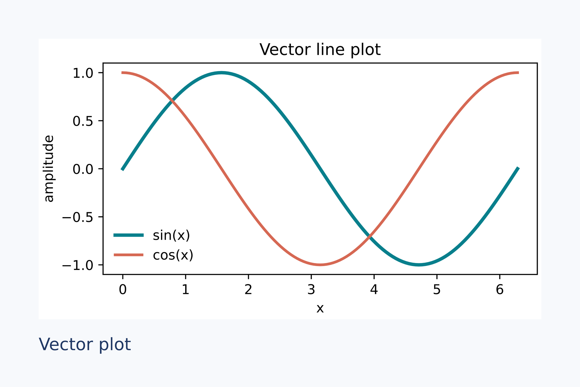
Dependencies

examples/gallery/notebook/vector.assets/fig-db872339bf178acf.svg
examples/gallery/notebook/vector.lay

Parameters#

Parameter	Purpose	Default or requirement
`--dpi`	Final PNG resolution	Does not control the Figure asset
`--plot-dpi`	Figure fallback PNG resolution	300

Workflow#

This workflow keeps an existing Matplotlib figure and places it on a LayMesh page.

Compute data and make a Figure in Python:

1import numpy as np2import pandas as pd3import matplotlib.pyplot as plt4 5x = np.linspace(0, 2 * np.pi, 100)6df = pd.DataFrame({"x": x, "y": np.sin(x)})7fig, ax = plt.subplots(figsize=(4, 2.5))8ax.plot(df["x"], df["y"])9title = f"Peak: {df['y'].max():.2f}"

import numpy as np
import pandas as pd
import matplotlib.pyplot as plt

x = np.linspace(0, 2 * np.pi, 100)
df = pd.DataFrame({"x": x, "y": np.sin(x)})
fig, ax = plt.subplots(figsize=(4, 2.5))
ax.plot(df["x"], df["y"])
title = f"Peak: {df['y'].max():.2f}"

Load the extension and put .lay directly in the next cell:

1%load_ext laymesh.ipython

%load_ext laymesh.ipython

1%%laymesh -o figure.pdf --save-source figure.lay2page = canvas(size=(160 mm, 100 mm), background="#ffffff")3chart = image(src={{fig}})4placed = page.add(chart,size=(130 mm, auto),5                  target=page.top_left, offset=(15 mm, 10 mm))6caption = text(content={{title}}, font_size=10 pt)7page.add(caption, target=placed.bottom_left, offset=(0 mm, 4 mm))

%%laymesh -o figure.pdf --save-source figure.lay
page = canvas(size=(160 mm, 100 mm), background="#ffffff")
chart = image(src={{fig}})
placed = page.add(chart,size=(130 mm, auto),
                  target=page.top_left, offset=(15 mm, 10 mm))
caption = text(content={{title}}, font_size=10 pt)
page.add(caption, target=placed.bottom_left, offset=(0 mm, 4 mm))

The cell displays an SVG preview and exports figure.pdf. --save-source figure.lay also saves the expanded layout and plot asset in figure.assets/; outside the Notebook you can run laymesh render figure.lay -o another.pdf. Repeated execution overwrites only .lay files carrying a LayMesh-generated marker, not handwritten layouts. Saved assets have content-hash names; obsolete ones may remain. Omit --save-source when the Notebook itself is sufficient as the reproducible source.

Use line magic for an existing layout:

1%laymesh figures/layout.lay -o figures/output.png --dpi 300

%laymesh figures/layout.lay -o figures/output.png --dpi 300

Relative image, font, and module paths then resolve beside layout.lay. In %%laymesh, they resolve from the Notebook process's working directory; check Path.cwd() in Python. -o supports SVG, PDF, and PNG; without it, only a temporary preview is produced. --dpi controls final PNG pixels. --plot-dpi (default 300) controls only a Matplotlib figure that must fall back to a raster asset.

An unquoted {{name}} refers to one Notebook variable. Supported values include strings, booleans, finite scalars, Path, Matplotlib Figures, numeric lists, 1D/2D ndarrays, Series and DataFrames. Arrays and tables become portable JSON assets for native plotting. NaN/None/pandas NA represent missing values; infinity is rejected. Undefined names and Python expressions remain unsupported.

Supported Matplotlib line plots stay as SVG vector artwork. Matplotlib normally converts labels into vector paths, which look stable but are not selectable text. Heatmaps or other content outside LayMesh's safe SVG subset fall back to PNG with a Notebook warning. Text created by LayMesh itself retains its usual export behavior. External SVG files do not use this Matplotlib adapter; they still undergo the normal SVG security checks.

W_PLOT_BOUNDS means visible Figure content extends outside the original canvas. Jupyter's inline preview may use tight bounds and still show an outlying axis title; LayMesh exports the Figure's original bounds and may clip it. The warning names the affected direction. LayMesh does not silently resize the plot. Call fig.tight_layout() or create it with layout="constrained", then rerun the magic.

Ordinary Python scripts use the same bridge:

1from laymesh import render_source2 3result = render_source(4    r"""page=canvas(size=(100 mm,70 mm))5chart=image(src={{fig}})6page.add(chart,size=(80 mm, auto),target=page.center,anchor=center)7""",8    namespace={"fig": fig},9    output="figure.pdf",10)11print(result.output)

from laymesh import render_source

result = render_source(
    r"""page=canvas(size=(100 mm,70 mm))
chart=image(src={{fig}})
page.add(chart,size=(80 mm, auto),target=page.center,anchor=center)
""",
    namespace={"fig": fig},
    output="figure.pdf",
)
print(result.output)

render_file("layout.lay", namespace={...}, output="figure.pdf") performs the same process on an existing source file. Both functions return SVG preview text, the optional output path, and an optional saved-source path.

The full example Notebook covers line plots, heatmaps, and rerendering saved source. See the Notebook gallery for actual assets, fallback messages, and both DPI settings.

Native arrays and DataFrames · Notebook Magic · Save source and render independently

workflow#

Complete sources and executable verification fixtures for this workflow are listed in the feature coverage map. Follow this page’s input conditions and limits when composing features.

Matplotlib import#

Parameters#

Workflow#

Limits and related topics#

workflow#