Lines and scatter#

Purpose and concepts#

line connects valid points; scatter draws markers only. Both retain input order. line’s marker can expose samples, and physical style sizes are independent of data domains.

Minimal complete example#

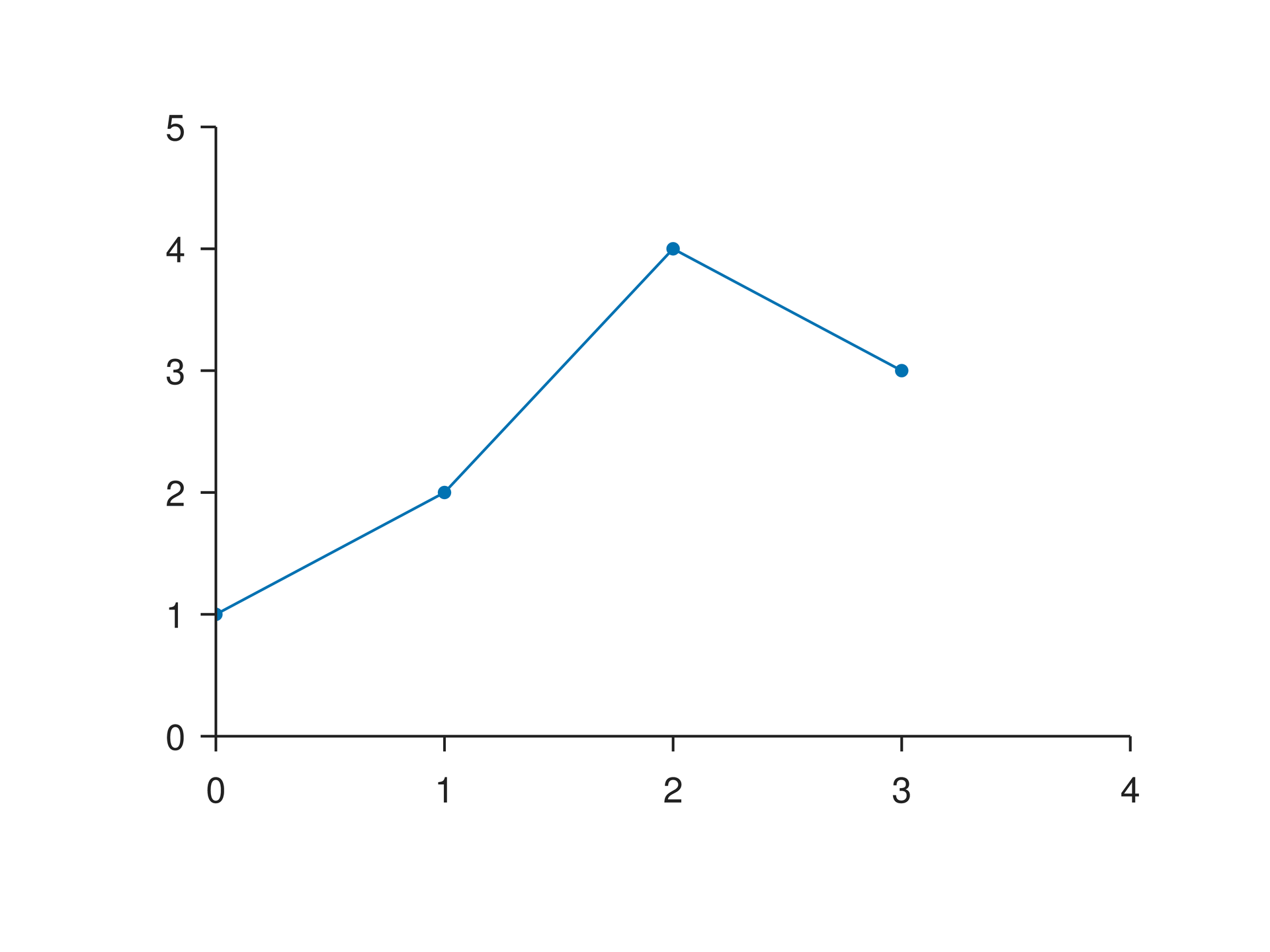
Run this file directly with laymesh validate or laymesh render; it contains its own canvas and required definitions.

1# Minimal complete example: plot.line2page=canvas(size=(100mm,75mm),background="#ffffff")3p=plot(size=(86mm,62mm),x=axis(range=(0,4)),y=axis(range=(0,5)))4p.line(x=[0,1,2,3],y=[1,2,4,3],marker=circle)5page.add(p,offset=(7mm,6mm))

# Minimal complete example: plot.line
page=canvas(size=(100mm,75mm),background="#ffffff")
p=plot(size=(86mm,62mm),x=axis(range=(0,4)),y=axis(range=(0,5)))
p.line(x=[0,1,2,3],y=[1,2,4,3],marker=circle)
page.add(p,offset=(7mm,6mm))

1# Minimal complete example: plot.line2page=canvas(size=(100mm,75mm),background="#ffffff")3p=plot(size=(86mm,62mm),x=axis(range=(0,4)),y=axis(range=(0,5)))4p.line(x=[0,1,2,3],y=[1,2,4,3],marker=circle)5page.add(p,offset=(7mm,6mm))

# Minimal complete example: plot.line
page=canvas(size=(100mm,75mm),background="#ffffff")
p=plot(size=(86mm,62mm),x=axis(range=(0,4)),y=axis(range=(0,5)))
p.line(x=[0,1,2,3],y=[1,2,4,3],marker=circle)
page.add(p,offset=(7mm,6mm))

Dependencies

examples/manual/plot-line.lay

Parameters and default behavior#

Unitless geometry uses the canvas unit; unitless type and stroke sizes use pt. Explicit call parameters override inherited/theme defaults. The linked interface reference lists accepted types, choices and defaults per parameter.

Composition#

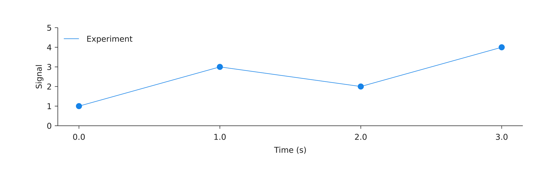
Connect x/y with a light line and emphasize points with markers. scatter’s c plus color_scale shows a third variable; marker_size and opacity can be arrays matching data length.

4p = plot(size=(210 mm, 58 mm), plot_area=box(offset=(18 mm, 6 mm), size=(185 mm, 39 mm)),5         x=axis(label="Time (s)", range=(-0.15, 3.15), ticks=[0, 1, 2, 3]),6         y=axis(label="Signal", range=(0, 5)), style=style)7p.line(x=[0, 1, 2, 3], y=[1, 3, 2, 4], color="#1683e8", label="Experiment")8p.scatter(x=[0, 1, 2, 3], y=[1, 3, 2, 4], color="#1683e8", marker_size=2.4 mm)9p.legend(position= top_left)10page.add(p, offset=(5 mm, 5 mm))

p = plot(size=(210 mm, 58 mm), plot_area=box(offset=(18 mm, 6 mm), size=(185 mm, 39 mm)),
         x=axis(label="Time (s)", range=(-0.15, 3.15), ticks=[0, 1, 2, 3]),
         y=axis(label="Signal", range=(0, 5)), style=style)
p.line(x=[0, 1, 2, 3], y=[1, 3, 2, 4], color="#1683e8", label="Experiment")
p.scatter(x=[0, 1, 2, 3], y=[1, 3, 2, 4], color="#1683e8", marker_size=2.4 mm)
p.legend(position= top_left)
page.add(p, offset=(5 mm, 5 mm))

1page = canvas(size=(220 mm, 68 mm), background="#ffffff")2style = plot_style(font_family="DejaVu Sans", font_size=9 pt)3# BEGIN DEMO4p = plot(size=(210 mm, 58 mm), plot_area=box(offset=(18 mm, 6 mm), size=(185 mm, 39 mm)),5         x=axis(label="Time (s)", range=(-0.15, 3.15), ticks=[0, 1, 2, 3]),6         y=axis(label="Signal", range=(0, 5)), style=style)7p.line(x=[0, 1, 2, 3], y=[1, 3, 2, 4], color="#1683e8", label="Experiment")8p.scatter(x=[0, 1, 2, 3], y=[1, 3, 2, 4], color="#1683e8", marker_size=2.4 mm)9p.legend(position= top_left)10page.add(p, offset=(5 mm, 5 mm))11# END DEMO

page = canvas(size=(220 mm, 68 mm), background="#ffffff")
style = plot_style(font_family="DejaVu Sans", font_size=9 pt)
# BEGIN DEMO
p = plot(size=(210 mm, 58 mm), plot_area=box(offset=(18 mm, 6 mm), size=(185 mm, 39 mm)),
         x=axis(label="Time (s)", range=(-0.15, 3.15), ticks=[0, 1, 2, 3]),
         y=axis(label="Signal", range=(0, 5)), style=style)
p.line(x=[0, 1, 2, 3], y=[1, 3, 2, 4], color="#1683e8", label="Experiment")
p.scatter(x=[0, 1, 2, 3], y=[1, 3, 2, 4], color="#1683e8", marker_size=2.4 mm)
p.legend(position= top_left)
page.add(p, offset=(5 mm, 5 mm))
# END DEMO

Dependencies

examples/plot/line-scatter.lay

Common errors and limits#

x is not automatically sorted. c and marker_fill are exclusive; per-point arrays must match. Missing samples break lines or skip markers. Supported markers are circle/square/triangle/triangle_down/diamond/none.

Individual functions#

plot-line#

Add a line layer connecting data points in order, optionally with markers. Choose named axes with x_axis and y_axis; polar plots use theta and r, and radar plots use values.

Returns: A layer handle that can be included in a shared legend.

Minimal complete source · Composition source · All parameters

plot-scatter#

Add a scatter layer. Set marker shape, physical size and border, or map numeric c values to colors through color_scale.

Returns: A layer handle that can be included in a shared legend.

Minimal complete source · Composition source · All parameters

Detailed behavior and further examples#

Parameters#

Parameter	Purpose	Default or requirement
`x / y`	Equal-length data sequences	Required
`marker_size`	Physical marker size	Example: 2.4 mm
`label`	Legend text	Optional

Common usage#

line connects data in input order without sorting; scatter draws individual observations. Overlay them using the same axes and color. Lines break at missing values and scatter skips them.

Complete parameters and rules

Error bars and bands · Bars and steps · Heatmaps and contours · Multiple axes and breaks