 LayMesh
Radar charts#
Purpose and concepts#
radar assigns each category an angle and its own domain, normalizing values into a common physical radius. It compares multi-metric shapes without implying that different units have equal meaning.
Minimal complete example#
Run this file directly with laymesh validate or laymesh render; it contains its own canvas and required definitions.
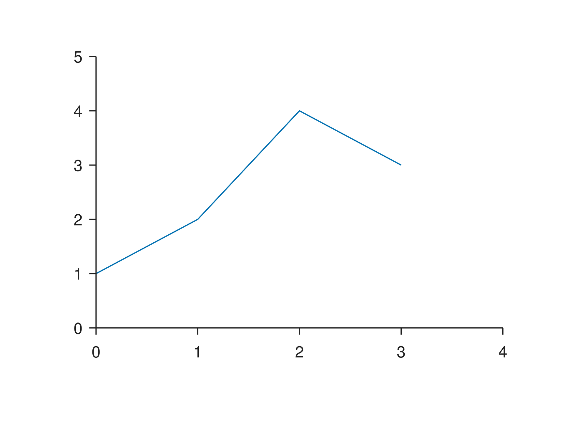
# Minimal complete example: plotpage=canvas(size=(100mm,75mm),background="#ffffff")p=plot(size=(86mm,62mm),x=axis(range=(0,4)),y=axis(range=(0,5)))p.line(x=[0,1,2,3],y=[1,2,4,3],label="Signal")page.add(p,offset=(7mm,6mm))# Minimal complete example: plotpage=canvas(size=(100mm,75mm),background="#ffffff")p=plot(size=(86mm,62mm),x=axis(range=(0,4)),y=axis(range=(0,5)))p.line(x=[0,1,2,3],y=[1,2,4,3],label="Signal")page.add(p,offset=(7mm,6mm))Preview
Dependencies
examples/manual/plot.lay
Parameters and default behavior#
Unitless geometry uses the canvas unit; unitless type and stroke sizes use pt. Explicit call parameters override inherited/theme defaults. The linked interface reference lists accepted types, choices and defaults per parameter.
Composition#
Match categories with ranges and use closed=true line or area to join endpoints. Original-data anchors accept category/value; labels use categories or separate text.
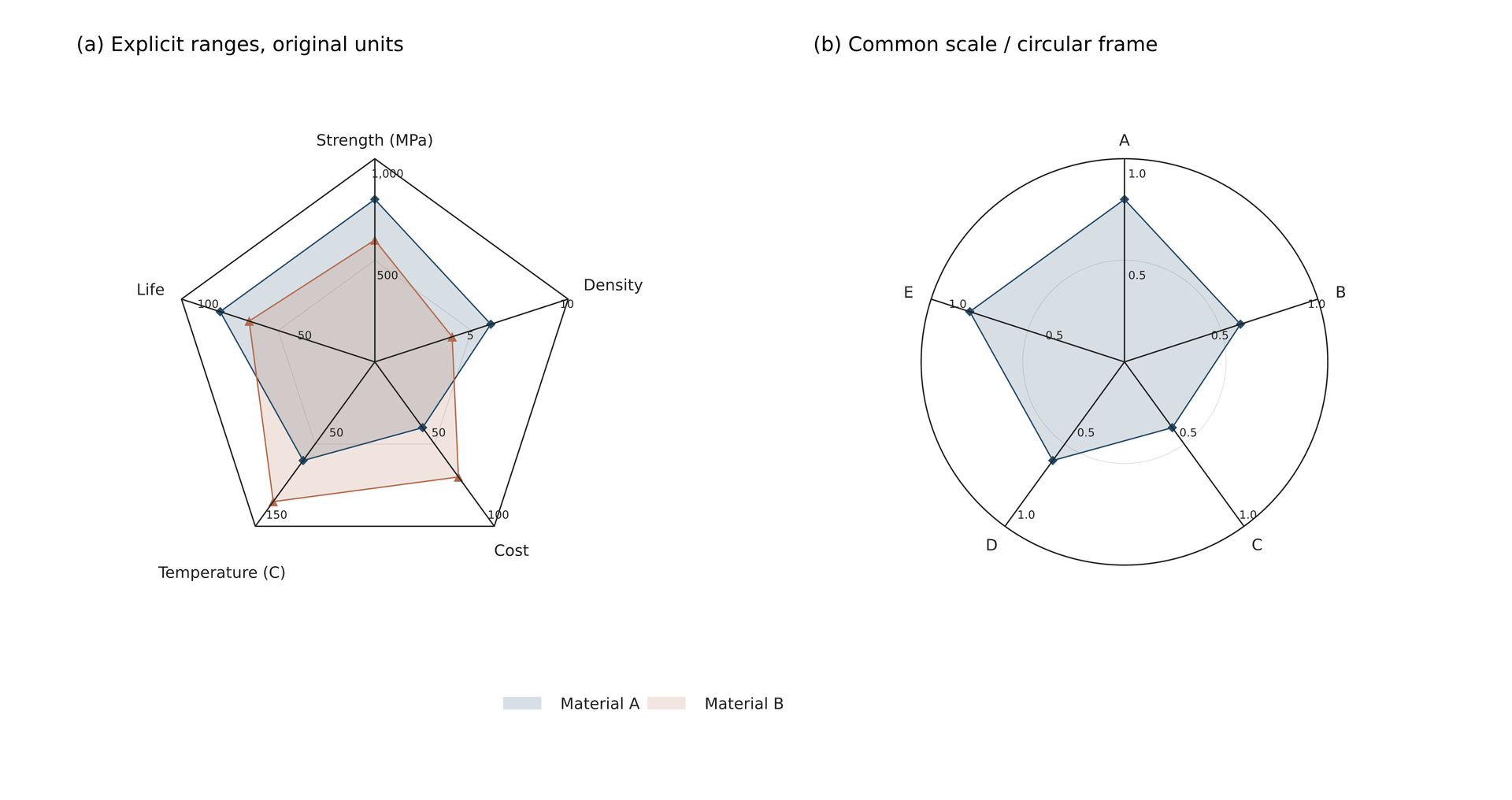
page=canvas(size=(238 mm,126 mm),background="#ffffff")s=plot_style(font_family="DejaVu Sans",font_size=7 pt)p=plot(projection= radar,size=(115 mm,110 mm),plot_area=box(offset=(25 mm, 25 mm), size=(64 mm, 64 mm)),style=s, categories=["Strength","Density","Cost","Temperature","Life"], category_labels=["Strength (MPa)","Density", "Cost", "Temperature (C)","Life"], ranges=[(0,1000),(0,10),(0,100),(-50,150),(0,100)],r=axis(ticks=[0.5,1],grid= major,tick_font_size=5 pt))a=p.area(values=[800,6,40,70,80],fill="#264b69",color="#264b69",opacity=0.18,label="Material A")b=p.area(values=[600,4,70,120,65],fill="#b46c50",color="#b46c50",opacity=0.18,label="Material B")p.line(values=[800,6,40,70,80],marker= diamond,marker_size=1.5 mm,color="#264b69")p.line(values=[600,4,70,120,65],marker= triangle,marker_size=1.5 mm,color="#b46c50")c=page.add(p,offset=(2 mm,0 mm))page.add(text(content="(a) Explicit ranges, original units",font_family="DejaVu Sans",font_size=9 pt),offset=(12 mm,5 mm))q=plot(projection= radar,size=(115 mm,110 mm),plot_area=box(offset=(25 mm, 25 mm), size=(64 mm, 64 mm)),style=s,categories=["A","B","C","D","E"],radar_frame="circle",r=axis(range=(0,1),ticks=[0.5,1],grid= major,tick_font_size=5 pt))q.area(values=[0.8,0.6,0.4,0.6,0.8],fill="#264b69",opacity=0.18)q.line(values=[0.8,0.6,0.4,0.6,0.8],marker= diamond,marker_size=1.5 mm,color="#264b69")d=page.add(q,offset=(120 mm,0 mm))page.add(text(content="(b) Common scale / circular frame",font_family="DejaVu Sans",font_size=9 pt),offset=(128 mm,5 mm))page.add(legend(layers=[a,b],columns=2,style=s),offset=(78 mm,108 mm))# BEGIN DEMOpage=canvas(size=(238 mm,126 mm),background="#ffffff")s=plot_style(font_family="DejaVu Sans",font_size=7 pt)p=plot(projection= radar,size=(115 mm,110 mm),plot_area=box(offset=(25 mm, 25 mm), size=(64 mm, 64 mm)),style=s, categories=["Strength","Density","Cost","Temperature","Life"], category_labels=["Strength (MPa)","Density", "Cost", "Temperature (C)","Life"], ranges=[(0,1000),(0,10),(0,100),(-50,150),(0,100)],r=axis(ticks=[0.5,1],grid= major,tick_font_size=5 pt))a=p.area(values=[800,6,40,70,80],fill="#264b69",color="#264b69",opacity=0.18,label="Material A")b=p.area(values=[600,4,70,120,65],fill="#b46c50",color="#b46c50",opacity=0.18,label="Material B")p.line(values=[800,6,40,70,80],marker= diamond,marker_size=1.5 mm,color="#264b69")p.line(values=[600,4,70,120,65],marker= triangle,marker_size=1.5 mm,color="#b46c50")c=page.add(p,offset=(2 mm,0 mm))page.add(text(content="(a) Explicit ranges, original units",font_family="DejaVu Sans",font_size=9 pt),offset=(12 mm,5 mm))q=plot(projection= radar,size=(115 mm,110 mm),plot_area=box(offset=(25 mm, 25 mm), size=(64 mm, 64 mm)),style=s,categories=["A","B","C","D","E"],radar_frame="circle",r=axis(range=(0,1),ticks=[0.5,1],grid= major,tick_font_size=5 pt))q.area(values=[0.8,0.6,0.4,0.6,0.8],fill="#264b69",opacity=0.18)q.line(values=[0.8,0.6,0.4,0.6,0.8],marker= diamond,marker_size=1.5 mm,color="#264b69")d=page.add(q,offset=(120 mm,0 mm))page.add(text(content="(b) Common scale / circular frame",font_family="DejaVu Sans",font_size=9 pt),offset=(128 mm,5 mm))page.add(legend(layers=[a,b],columns=2,style=s),offset=(78 mm,108 mm))# END DEMOPreview
Dependencies
examples/plot/radar.lay
Common errors and limits#
Category order is not inferred. Each series must match category count with valid domains and visible values. Continuous polar theta selection is not a category index.
Individual functions#
Detailed behavior and further examples#
Parameters#
| Parameter | Purpose | Default or requirement |
|---|---|---|
categories |
Categories and order | Explicitly specified |
range |
Radial data range | Linear and non-reversed |
Common usage#
At least three unique categories retain input order, equally spaced, starting at the top clockwise by default. category_labels accepts matching rich labels. radar_frame="polygon|circle" defaults to polygon with aligned grid vertices. line/scatter/area(values=...) accept matching arrays; lines and areas close by default and use straight edges.
Without ranges, every category shares r.range, or one automatic range computed across all series. Explicit ranges normalizes each indicator linearly and conflicts with a common r.range. In this mode r.ticks specifies common 0–1 positions while displayed values use each indicator's original units. With offset notation and independent ranges, each spoke displays its own multiplier. Negative original values inside their ranges keep their category direction. Out-of-range values error; missing values break lines and suppress the affected series' closed area.
a.data(category=...,value=...) uses raw units; a.axis(name=category,anchor=...) references a spoke. Radar uses linear, non-reversed scales, with no theta axis, inner hole or breaks.