 LayMesh
Boxplots and violin plots#
Purpose and concepts#
boxplot summarizes quantiles, whiskers and outliers; violin shows a kernel density estimate. Both accept observations rather than an already summarized five-number result.
Minimal complete example#
Run this file directly with laymesh validate or laymesh render; it contains its own canvas and required definitions.
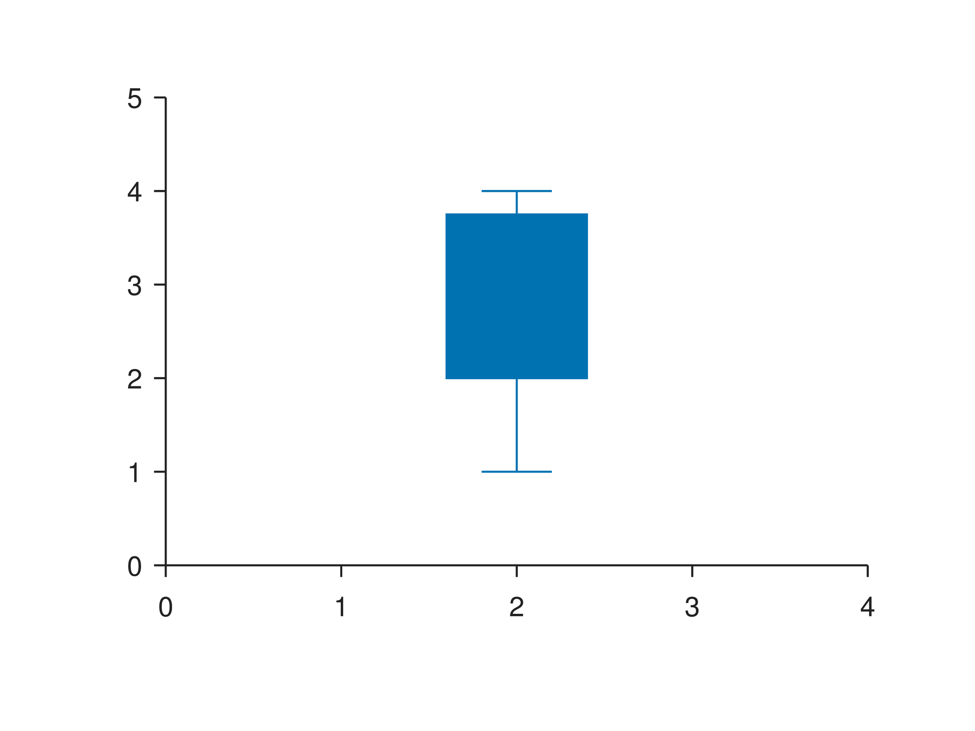
# Minimal complete example: plot.boxplotpage=canvas(size=(100mm,75mm),background="#ffffff")p=plot(size=(86mm,62mm),x=axis(range=(0,4)),y=axis(range=(0,5)))p.boxplot(values=[1,2,2,3,4,4],position=2)page.add(p,offset=(7mm,6mm))# Minimal complete example: plot.boxplotpage=canvas(size=(100mm,75mm),background="#ffffff")p=plot(size=(86mm,62mm),x=axis(range=(0,4)),y=axis(range=(0,5)))p.boxplot(values=[1,2,2,3,4,4],position=2)page.add(p,offset=(7mm,6mm))Preview
Dependencies
examples/manual/plot-boxplot.lay
Parameters and default behavior#
Unitless geometry uses the canvas unit; unitless type and stroke sizes use pt. Explicit call parameters override inherited/theme defaults. The linked interface reference lists accepted types, choices and defaults per parameter.
Composition#
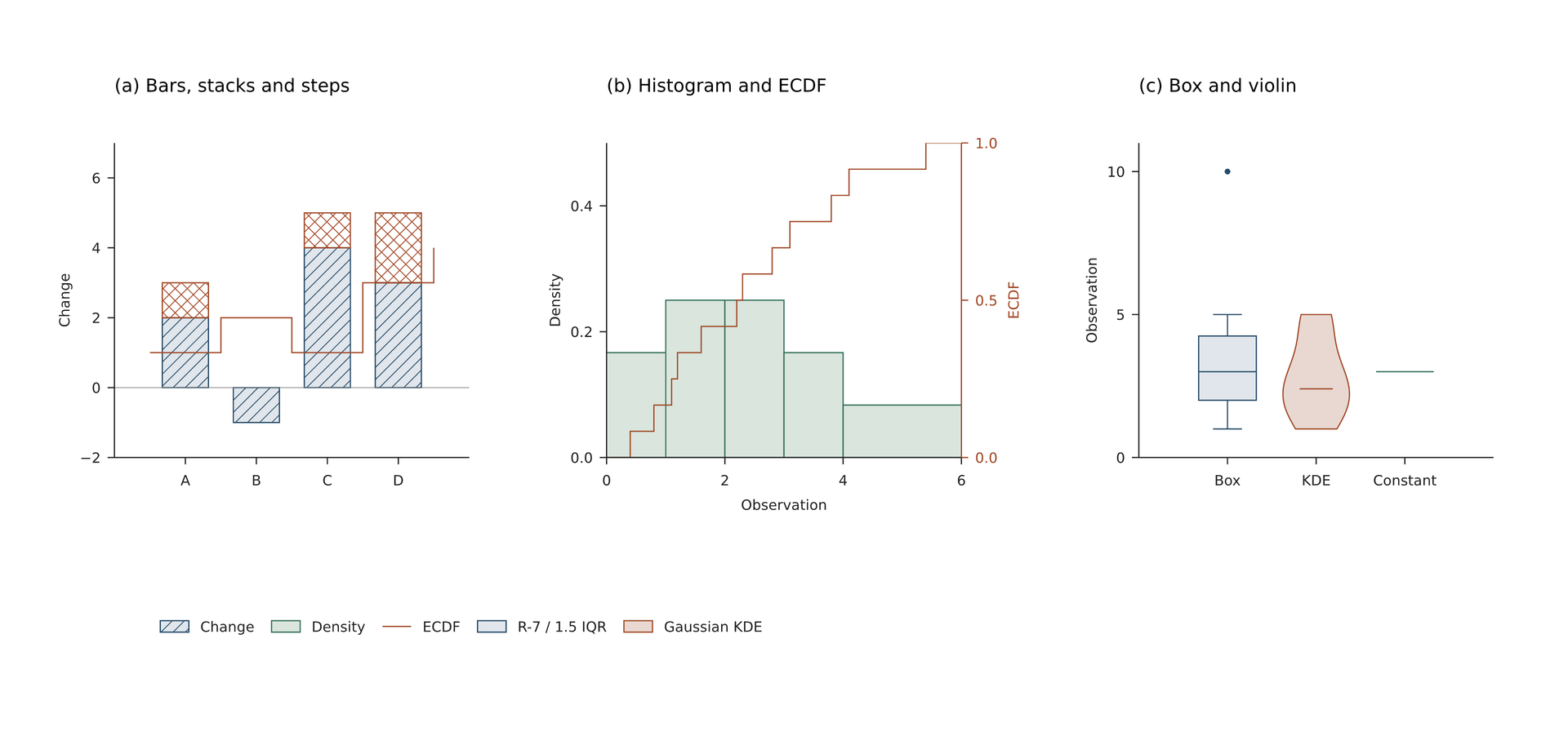
Place boxplot and violin for one sample at neighboring positions with explicit data_width. R-7 quantiles, default 1.5 IQR whiskers and Scott bandwidth specify the statistical convention.
# Statistics are evaluated in original data units. Positions preserve input order.page=canvas(size=(274 mm,128 mm),background="#ffffff")s=plot_style(font_family="DejaVu Sans",font_size=7 pt)a=plot(size=(88 mm,91 mm),plot_area=box(offset=(16 mm, 15 mm), size=(62 mm, 55 mm)),style=s, x=axis(range=(0,5),ticks=[1,2,3,4],tick_text=["A","B","C","D"]),y=axis(label="Change",range=(-2,7),ticks=[-2,0,2,4,6]))bar=a.bar(positions=[1,2,3,4],values=[2,-1,4,3],data_width=0.65,fill="#e0e6eb",border_color="#264b69",hatch="slash",hatch_spacing=1.5 mm,label="Change")a.bar(positions=[1,3,4],values=[1,1,2],baseline=[2,4,3],data_width=0.65,fill="none",border_color="#a04725",hatch="cross",label="Stack")a.hline(y=0,color="#777777",line_width=0.3 pt)a.step(x=[0.5,1.5,2.5,3.5,4.5],y=[1,2,1,3,4],where= post,color="#a04725")ca=page.add(a,offset=(4 mm,10 mm))page.add(text(content="(a) Bars, stacks and steps",font_family="DejaVu Sans",font_size=9 pt),target=ca.plot_top_left,offset=(0 mm,-12 mm)) b=plot(size=(104 mm,91 mm),plot_area=box(offset=(16 mm, 15 mm), size=(62 mm, 55 mm)),style=s, x=axis(label="Observation",range=(0,6),ticks=[0,2,4,6]),y=axis(label="Density",range=(0,0.5),ticks=[0,0.2,0.4]))b.add_axis(name="cumulative",side= right,axis=axis(label="ECDF",range=(0,1),ticks=[0,0.5,1],line_color="#a04725"))hist=b.hist(values=[0.4,0.8,1.1,1.2,1.6,2.2,2.3,2.8,3.1,3.8,4.1,5.4],bins=[0,1,2,3,4,6],stat= density,fill="#d9e5dd",border_color="#34705a",label="Density")ecdf=b.ecdf(values=[0.4,0.8,1.1,1.2,1.6,2.2,2.3,2.8,3.1,3.8,4.1,5.4],y_axis="cumulative",color="#a04725",label="ECDF")cb=page.add(b,offset=(90 mm,10 mm))page.add(text(content="(b) Histogram and ECDF",font_family="DejaVu Sans",font_size=9 pt),target=cb.plot_top_left,offset=(0 mm,-12 mm)) c=plot(size=(88 mm,91 mm),plot_area=box(offset=(20 mm, 15 mm), size=(62 mm, 55 mm)),style=s, x=axis(range=(0,4),ticks=[1,2,3],tick_text=["Box","KDE","Constant"]),y=axis(label="Observation",range=(0,11),ticks=[0,5,10]))box=c.boxplot(values=[1,2,2,3,3,4,5,10],position=1,data_width=0.65,fill="#e0e6eb",border_color="#264b69",label="R-7 / 1.5 IQR")violin=c.violin(values=[1,1.5,2,2.2,2.4,3,3.5,4.8,5],position=2,data_width=0.75,fill="#e8d8d1",border_color="#a04725",label="Gaussian KDE")c.violin(values=[3,3,3],position=3,data_width=0.65,color="#34705a")cc=page.add(c,offset=(179 mm,10 mm))page.add(text(content="(c) Box and violin",font_family="DejaVu Sans",font_size=9 pt),target=cc.plot_top_left,offset=(0 mm,-12 mm))page.add(legend(layers=[bar,hist,ecdf,box,violin],columns=5,gap=3 mm,background="none",sample_width=5 mm,sample_gap=2 mm),offset=(25 mm,105 mm))# BEGIN DEMO# Statistics are evaluated in original data units. Positions preserve input order.page=canvas(size=(274 mm,128 mm),background="#ffffff")s=plot_style(font_family="DejaVu Sans",font_size=7 pt)a=plot(size=(88 mm,91 mm),plot_area=box(offset=(16 mm, 15 mm), size=(62 mm, 55 mm)),style=s, x=axis(range=(0,5),ticks=[1,2,3,4],tick_text=["A","B","C","D"]),y=axis(label="Change",range=(-2,7),ticks=[-2,0,2,4,6]))bar=a.bar(positions=[1,2,3,4],values=[2,-1,4,3],data_width=0.65,fill="#e0e6eb",border_color="#264b69",hatch="slash",hatch_spacing=1.5 mm,label="Change")a.bar(positions=[1,3,4],values=[1,1,2],baseline=[2,4,3],data_width=0.65,fill="none",border_color="#a04725",hatch="cross",label="Stack")a.hline(y=0,color="#777777",line_width=0.3 pt)a.step(x=[0.5,1.5,2.5,3.5,4.5],y=[1,2,1,3,4],where= post,color="#a04725")ca=page.add(a,offset=(4 mm,10 mm))page.add(text(content="(a) Bars, stacks and steps",font_family="DejaVu Sans",font_size=9 pt),target=ca.plot_top_left,offset=(0 mm,-12 mm)) b=plot(size=(104 mm,91 mm),plot_area=box(offset=(16 mm, 15 mm), size=(62 mm, 55 mm)),style=s, x=axis(label="Observation",range=(0,6),ticks=[0,2,4,6]),y=axis(label="Density",range=(0,0.5),ticks=[0,0.2,0.4]))b.add_axis(name="cumulative",side= right,axis=axis(label="ECDF",range=(0,1),ticks=[0,0.5,1],line_color="#a04725"))hist=b.hist(values=[0.4,0.8,1.1,1.2,1.6,2.2,2.3,2.8,3.1,3.8,4.1,5.4],bins=[0,1,2,3,4,6],stat= density,fill="#d9e5dd",border_color="#34705a",label="Density")ecdf=b.ecdf(values=[0.4,0.8,1.1,1.2,1.6,2.2,2.3,2.8,3.1,3.8,4.1,5.4],y_axis="cumulative",color="#a04725",label="ECDF")cb=page.add(b,offset=(90 mm,10 mm))page.add(text(content="(b) Histogram and ECDF",font_family="DejaVu Sans",font_size=9 pt),target=cb.plot_top_left,offset=(0 mm,-12 mm)) c=plot(size=(88 mm,91 mm),plot_area=box(offset=(20 mm, 15 mm), size=(62 mm, 55 mm)),style=s, x=axis(range=(0,4),ticks=[1,2,3],tick_text=["Box","KDE","Constant"]),y=axis(label="Observation",range=(0,11),ticks=[0,5,10]))box=c.boxplot(values=[1,2,2,3,3,4,5,10],position=1,data_width=0.65,fill="#e0e6eb",border_color="#264b69",label="R-7 / 1.5 IQR")violin=c.violin(values=[1,1.5,2,2.2,2.4,3,3.5,4.8,5],position=2,data_width=0.75,fill="#e8d8d1",border_color="#a04725",label="Gaussian KDE")c.violin(values=[3,3,3],position=3,data_width=0.65,color="#34705a")cc=page.add(c,offset=(179 mm,10 mm))page.add(text(content="(c) Box and violin",font_family="DejaVu Sans",font_size=9 pt),target=cc.plot_top_left,offset=(0 mm,-12 mm))page.add(legend(layers=[bar,hist,ecdf,box,violin],columns=5,gap=3 mm,background="none",sample_width=5 mm,sample_gap=2 mm),offset=(25 mm,105 mm))# END DEMOPreview
Dependencies
examples/plot/statistics.lay
Common errors and limits#
Single/constant samples cannot form an ordinary violin density and show a median with a warning. points controls estimate sampling, not the observation count; it does not change data.
Individual functions#
plot-boxplot#
Box plot layer: add data to this plot, control its appearance with physical style parameters, and select data mappings with named-axis parameters.
Returns: A layer handle that can be included in a shared legend.
Minimal complete source · Composition source · All parameters
plot-violin#
Violin plot layer: add data to this plot, control its appearance with physical style parameters, and select data mappings with named-axis parameters.
Returns: A layer handle that can be included in a shared legend.
Minimal complete source · Composition source · All parameters
Detailed behavior and further examples#
Parameters#
| Parameter | Purpose | Default or requirement |
|---|---|---|
whisker |
Boxplot whisker IQR multiplier | 1.5 |
bandwidth |
KDE bandwidth | scott |
points |
Violin sample count | 128 |
Common usage#
Boxplots use R-7 quantiles and default whiskers reaching the most distant observation within 1.5 IQR. Violins use a Gaussian kernel and Scott bandwidth; constant or single-point samples show only the median with a warning.