 LayMesh
Data input and missing values#
Purpose and concepts#
Data values differ from physical dimensions: x/y are scalar axis values, while stroke widths and marker_size are physical lengths. Inline lists suit small samples; table reads CSV/column JSON and array reads JSON vectors/matrices.
Minimal complete example#
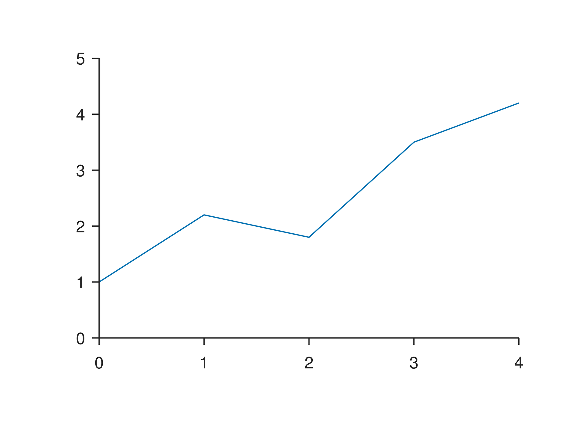
Run this file directly with laymesh validate or laymesh render; it contains its own canvas and required definitions.
# Minimal complete example: tablepage=canvas(size=(100mm,75mm),background="#ffffff")d=table(src="../plot/first-plot.csv")p=plot(size=(86mm,62mm),x=axis(range=(0,4)),y=axis(range=(0,5)))p.line(x=d["time"],y=d["signal"])page.add(p,offset=(7mm,6mm))# Minimal complete example: tablepage=canvas(size=(100mm,75mm),background="#ffffff")d=table(src="../plot/first-plot.csv")p=plot(size=(86mm,62mm),x=axis(range=(0,4)),y=axis(range=(0,5)))p.line(x=d["time"],y=d["signal"])page.add(p,offset=(7mm,6mm))time,signal,error0,1.0,0.21,2.2,0.32,1.8,0.23,3.5,0.44,4.2,0.3Preview
Dependencies
examples/manual/table.layexamples/plot/first-plot.csv
Parameters and default behavior#
Unitless geometry uses the canvas unit; unitless type and stroke sizes use pt. Explicit call parameters override inherited/theme defaults. The linked interface reference lists accepted types, choices and defaults per parameter.
Composition#
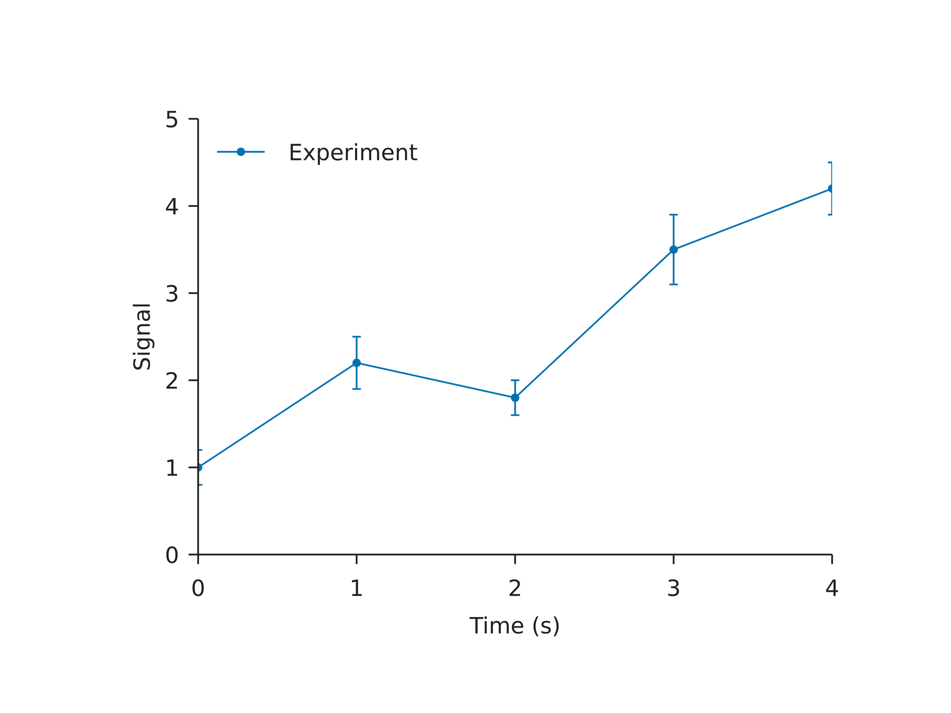
Reuse table columns for lines, errors and bands. Python DataFrame binding creates data resources that a saved layout can read through the CLI. null retains missingness without automatic interpolation.
page = canvas(size=(120 mm, 90 mm), background="#ffffff")d = table(src="first-plot.csv")s = plot_style(font_family="DejaVu Sans", font_size=8 pt)p = plot(size=(110 mm, 80 mm), plot_area=box(offset=(20 mm, 10 mm), size=(80 mm, 55 mm)), x=axis(label="Time (s)", range=(0, 4)), y=axis(label="Signal", range=(0, 5)), style=s)p.line(x=d["time"], y=d["signal"], marker= circle, color="#0072B2", label="Experiment")p.errorbar(x=d["time"], y=d["signal"], yerr=d["error"], color="#0072B2")p.legend(position= top_left)chart = page.add(p, offset=(5 mm, 5 mm))page = canvas(size=(120 mm, 90 mm), background="#ffffff")d = table(src="first-plot.csv")s = plot_style(font_family="DejaVu Sans", font_size=8 pt)p = plot(size=(110 mm, 80 mm), plot_area=box(offset=(20 mm, 10 mm), size=(80 mm, 55 mm)), x=axis(label="Time (s)", range=(0, 4)), y=axis(label="Signal", range=(0, 5)), style=s)p.line(x=d["time"], y=d["signal"], marker= circle, color="#0072B2", label="Experiment")p.errorbar(x=d["time"], y=d["signal"], yerr=d["error"], color="#0072B2")p.legend(position= top_left)chart = page.add(p, offset=(5 mm, 5 mm))time,signal,error0,1.0,0.21,2.2,0.32,1.8,0.23,3.5,0.44,4.2,0.3Preview
Dependencies
examples/plot/first-plot.csvexamples/plot/first-plot.lay
Common errors and limits#
table requires unique nonempty names and equal column lengths. array does not accept values: write inline lists directly. Missing samples may break curves or skip markers and emit W_PLOT_MISSING.
Individual functions#
table#
Read CSV or column-oriented JSON with unique nonempty headers and equal column lengths. d["column"] selects a column; null and empty CSV cells retain missing values.
Returns: table
Required inputs: src.
Minimal complete source · Composition source · All parameters
array#
Read a nonempty numeric vector/matrix from JSON. Matrices must be rectangular; null is missing. Inline data uses lists rather than array(values=...).
Returns: number[] | number[][]
Required inputs: src.
Minimal complete source · Composition source · All parameters
Detailed behavior and further examples#
Parameters#
| Parameter | Purpose | Default or requirement |
|---|---|---|
table(src=...) |
CSV/JSON table | Access by column name |
null |
Missing value | Diagnostics retained |
Common usage#
table(src="results.csv") reads a CSV with unique nonempty headers, or column-oriented JSON such as {"x":[0,1],"y":[2,3],"sample":["A","B"]}. Columns must be nonempty and equally long. String columns are retained, but plotting requires numeric columns. Use d["column"] to select a column. CSV quoting and UTF-8 BOM are supported; empty cells are missing, literal NaN strings are not.
array(src="matrix.json") reads a nonempty numeric vector or rectangular matrix. JSON null represents missing values. Booleans, non-finite values and integers outside the JavaScript safe-integer range are rejected. Paths resolve against the defining .lay file, including modules. Data is cached within one compilation and read again on the next compilation.
Missing rows break lines/bands, skip scatter/error bars, or become transparent heatmap cells, with a counted W_PLOT_MISSING. Length mismatches, empty valid data, negative uncertainty, invalid log values, ragged matrices and impossible layouts are located errors. Ordinary layers preserve data order without imputation or sampling; statistical methods explicitly calculate the documented summaries.
Limits and related topics#
Plot area and physical size · Axes and ticks · Labels and scientific notation · Legends and shared colorbars · Data anchors and annotations