Projection and radial axes#

Purpose and concepts#

polar uses theta/r. Its default zero points right and positive direction is counterclockwise, unlike page line angles with downward y. angle_unit determines data-angle units.

Minimal complete example#

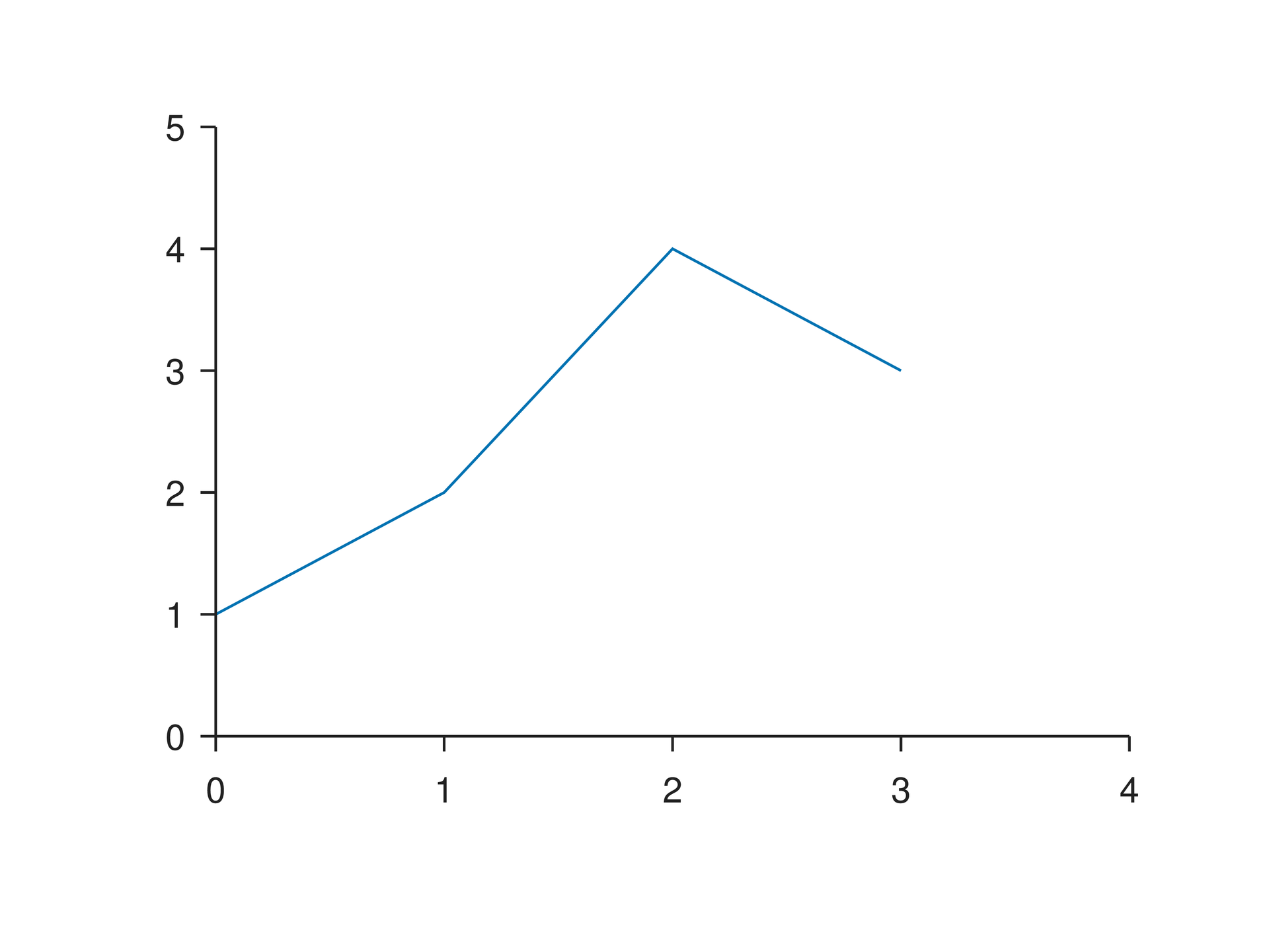
Run this file directly with laymesh validate or laymesh render; it contains its own canvas and required definitions.

1# Minimal complete example: plot2page=canvas(size=(100mm,75mm),background="#ffffff")3p=plot(size=(86mm,62mm),x=axis(range=(0,4)),y=axis(range=(0,5)))4p.line(x=[0,1,2,3],y=[1,2,4,3],label="Signal")5page.add(p,offset=(7mm,6mm))

# Minimal complete example: plot
page=canvas(size=(100mm,75mm),background="#ffffff")
p=plot(size=(86mm,62mm),x=axis(range=(0,4)),y=axis(range=(0,5)))
p.line(x=[0,1,2,3],y=[1,2,4,3],label="Signal")
page.add(p,offset=(7mm,6mm))

1# Minimal complete example: plot2page=canvas(size=(100mm,75mm),background="#ffffff")3p=plot(size=(86mm,62mm),x=axis(range=(0,4)),y=axis(range=(0,5)))4p.line(x=[0,1,2,3],y=[1,2,4,3],label="Signal")5page.add(p,offset=(7mm,6mm))

# Minimal complete example: plot
page=canvas(size=(100mm,75mm),background="#ffffff")
p=plot(size=(86mm,62mm),x=axis(range=(0,4)),y=axis(range=(0,5)))
p.line(x=[0,1,2,3],y=[1,2,4,3],label="Signal")
page.add(p,offset=(7mm,6mm))

Dependencies

examples/manual/plot.lay

Parameters and default behavior#

Unitless geometry uses the canvas unit; unitless type and stroke sizes use pt. Explicit call parameters override inherited/theme defaults. The linked interface reference lists accepted types, choices and defaults per parameter.

Composition#

theta_zero, theta_direction and inner_radius create gauges/rings. wrap=shortest crosses periods along the shortest route, while raw keeps angular differences. interpolation=polar/chord connects in data/page coordinates.

2page=canvas(size=(205 mm,120 mm),background="#ffffff")3s=plot_style(font_family="DejaVu Sans",font_size=7 pt,grid_color="#dddddd")4p=plot(projection= polar,size=(98 mm,100 mm),plot_area=box(offset=(18 mm, 18 mm), size=(62 mm, 62 mm)),style=s,5       theta=axis(ticks=[0,90,180,270],grid= major),r=axis(range=(0,5),ticks=[1,3,5],grid= major,tick_font_size=6 pt))6a=p.line(theta=[0,45,90,135,180,225,270,315],r=[4.5,3,1.6,2.5,4,2.8,1.3,3.4],closed=true,marker= diamond,marker_size=1.7 mm,color="#264b69",label="Response")7p.line(theta=[350,10],r=[4,4],color="#b65337",line_width=0.6 mm,label="350 to 10 degrees")8p.scatter(theta=[180],r=[-4.5],marker= circle,marker_size=3 mm,marker_fill="none",marker_border_color="#b65337",marker_border_width=0.3 mm)9c=page.add(p,offset=(3 mm,4 mm))10page.add(text(content="(a) Directional response",font_family="DejaVu Sans",font_size=9 pt),target=c.plot_top_left,offset=(-4 mm,-15 mm))11page.add(text(content="Peak",font_family="DejaVu Sans",font_size=7 pt),target=c.data(theta=0,r=4.5),offset=(-12 mm,-6 mm))12q=plot(projection= polar,size=(98 mm,100 mm),plot_area=box(offset=(18 mm, 18 mm), size=(62 mm, 62 mm)),style=s,theta_zero=90 deg,theta_direction="cw",13       theta=axis(ticks=[0,90,180,270],tick_text=["N","E","S","W"],grid= major),r=axis(range=(0,5),ticks=[1,3,5],grid= major,tick_font_size=6 pt))14q.line(theta=[0,45,90,135,180,225,270,315],r=[4.5,3,1.6,2.5,4,2.8,1.3,3.4],closed=true,marker= diamond,marker_size=1.7 mm,color="#264b69")15d=page.add(q,offset=(103 mm,4 mm))16page.add(text(content="(b) North / clockwise",font_family="DejaVu Sans",font_size=9 pt),target=d.plot_top_left,offset=(-4 mm,-15 mm))17page.add(legend(layers=[a],style=s),offset=(12 mm,103 mm))18page.add(text(content="Negative radius: same point after a half-turn (warning can be hidden).",font_family="DejaVu Sans",font_size=7 pt),offset=(53 mm,107 mm))

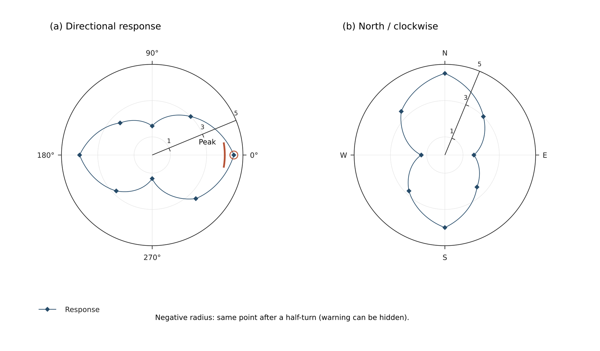
page=canvas(size=(205 mm,120 mm),background="#ffffff")
s=plot_style(font_family="DejaVu Sans",font_size=7 pt,grid_color="#dddddd")
p=plot(projection= polar,size=(98 mm,100 mm),plot_area=box(offset=(18 mm, 18 mm), size=(62 mm, 62 mm)),style=s,
       theta=axis(ticks=[0,90,180,270],grid= major),r=axis(range=(0,5),ticks=[1,3,5],grid= major,tick_font_size=6 pt))
a=p.line(theta=[0,45,90,135,180,225,270,315],r=[4.5,3,1.6,2.5,4,2.8,1.3,3.4],closed=true,marker= diamond,marker_size=1.7 mm,color="#264b69",label="Response")
p.line(theta=[350,10],r=[4,4],color="#b65337",line_width=0.6 mm,label="350 to 10 degrees")
p.scatter(theta=[180],r=[-4.5],marker= circle,marker_size=3 mm,marker_fill="none",marker_border_color="#b65337",marker_border_width=0.3 mm)
c=page.add(p,offset=(3 mm,4 mm))
page.add(text(content="(a) Directional response",font_family="DejaVu Sans",font_size=9 pt),target=c.plot_top_left,offset=(-4 mm,-15 mm))
page.add(text(content="Peak",font_family="DejaVu Sans",font_size=7 pt),target=c.data(theta=0,r=4.5),offset=(-12 mm,-6 mm))
q=plot(projection= polar,size=(98 mm,100 mm),plot_area=box(offset=(18 mm, 18 mm), size=(62 mm, 62 mm)),style=s,theta_zero=90 deg,theta_direction="cw",
       theta=axis(ticks=[0,90,180,270],tick_text=["N","E","S","W"],grid= major),r=axis(range=(0,5),ticks=[1,3,5],grid= major,tick_font_size=6 pt))
q.line(theta=[0,45,90,135,180,225,270,315],r=[4.5,3,1.6,2.5,4,2.8,1.3,3.4],closed=true,marker= diamond,marker_size=1.7 mm,color="#264b69")
d=page.add(q,offset=(103 mm,4 mm))
page.add(text(content="(b) North / clockwise",font_family="DejaVu Sans",font_size=9 pt),target=d.plot_top_left,offset=(-4 mm,-15 mm))
page.add(legend(layers=[a],style=s),offset=(12 mm,103 mm))
page.add(text(content="Negative radius: same point after a half-turn (warning can be hidden).",font_family="DejaVu Sans",font_size=7 pt),offset=(53 mm,107 mm))

1# BEGIN DEMO2page=canvas(size=(205 mm,120 mm),background="#ffffff")3s=plot_style(font_family="DejaVu Sans",font_size=7 pt,grid_color="#dddddd")4p=plot(projection= polar,size=(98 mm,100 mm),plot_area=box(offset=(18 mm, 18 mm), size=(62 mm, 62 mm)),style=s,5       theta=axis(ticks=[0,90,180,270],grid= major),r=axis(range=(0,5),ticks=[1,3,5],grid= major,tick_font_size=6 pt))6a=p.line(theta=[0,45,90,135,180,225,270,315],r=[4.5,3,1.6,2.5,4,2.8,1.3,3.4],closed=true,marker= diamond,marker_size=1.7 mm,color="#264b69",label="Response")7p.line(theta=[350,10],r=[4,4],color="#b65337",line_width=0.6 mm,label="350 to 10 degrees")8p.scatter(theta=[180],r=[-4.5],marker= circle,marker_size=3 mm,marker_fill="none",marker_border_color="#b65337",marker_border_width=0.3 mm)9c=page.add(p,offset=(3 mm,4 mm))10page.add(text(content="(a) Directional response",font_family="DejaVu Sans",font_size=9 pt),target=c.plot_top_left,offset=(-4 mm,-15 mm))11page.add(text(content="Peak",font_family="DejaVu Sans",font_size=7 pt),target=c.data(theta=0,r=4.5),offset=(-12 mm,-6 mm))12q=plot(projection= polar,size=(98 mm,100 mm),plot_area=box(offset=(18 mm, 18 mm), size=(62 mm, 62 mm)),style=s,theta_zero=90 deg,theta_direction="cw",13       theta=axis(ticks=[0,90,180,270],tick_text=["N","E","S","W"],grid= major),r=axis(range=(0,5),ticks=[1,3,5],grid= major,tick_font_size=6 pt))14q.line(theta=[0,45,90,135,180,225,270,315],r=[4.5,3,1.6,2.5,4,2.8,1.3,3.4],closed=true,marker= diamond,marker_size=1.7 mm,color="#264b69")15d=page.add(q,offset=(103 mm,4 mm))16page.add(text(content="(b) North / clockwise",font_family="DejaVu Sans",font_size=9 pt),target=d.plot_top_left,offset=(-4 mm,-15 mm))17page.add(legend(layers=[a],style=s),offset=(12 mm,103 mm))18page.add(text(content="Negative radius: same point after a half-turn (warning can be hidden).",font_family="DejaVu Sans",font_size=7 pt),offset=(53 mm,107 mm))19# END DEMO

# BEGIN DEMO
page=canvas(size=(205 mm,120 mm),background="#ffffff")
s=plot_style(font_family="DejaVu Sans",font_size=7 pt,grid_color="#dddddd")
p=plot(projection= polar,size=(98 mm,100 mm),plot_area=box(offset=(18 mm, 18 mm), size=(62 mm, 62 mm)),style=s,
       theta=axis(ticks=[0,90,180,270],grid= major),r=axis(range=(0,5),ticks=[1,3,5],grid= major,tick_font_size=6 pt))
a=p.line(theta=[0,45,90,135,180,225,270,315],r=[4.5,3,1.6,2.5,4,2.8,1.3,3.4],closed=true,marker= diamond,marker_size=1.7 mm,color="#264b69",label="Response")
p.line(theta=[350,10],r=[4,4],color="#b65337",line_width=0.6 mm,label="350 to 10 degrees")
p.scatter(theta=[180],r=[-4.5],marker= circle,marker_size=3 mm,marker_fill="none",marker_border_color="#b65337",marker_border_width=0.3 mm)
c=page.add(p,offset=(3 mm,4 mm))
page.add(text(content="(a) Directional response",font_family="DejaVu Sans",font_size=9 pt),target=c.plot_top_left,offset=(-4 mm,-15 mm))
page.add(text(content="Peak",font_family="DejaVu Sans",font_size=7 pt),target=c.data(theta=0,r=4.5),offset=(-12 mm,-6 mm))
q=plot(projection= polar,size=(98 mm,100 mm),plot_area=box(offset=(18 mm, 18 mm), size=(62 mm, 62 mm)),style=s,theta_zero=90 deg,theta_direction="cw",
       theta=axis(ticks=[0,90,180,270],tick_text=["N","E","S","W"],grid= major),r=axis(range=(0,5),ticks=[1,3,5],grid= major,tick_font_size=6 pt))
q.line(theta=[0,45,90,135,180,225,270,315],r=[4.5,3,1.6,2.5,4,2.8,1.3,3.4],closed=true,marker= diamond,marker_size=1.7 mm,color="#264b69")
d=page.add(q,offset=(103 mm,4 mm))
page.add(text(content="(b) North / clockwise",font_family="DejaVu Sans",font_size=9 pt),target=d.plot_top_left,offset=(-4 mm,-15 mm))
page.add(legend(layers=[a],style=s),offset=(12 mm,103 mm))
page.add(text(content="Negative radius: same point after a half-turn (warning can be hidden).",font_family="DejaVu Sans",font_size=7 pt),offset=(53 mm,107 mm))
# END DEMO

Dependencies

examples/plot/polar-directions.lay

Common errors and limits#

Negative radii add half a turn and use their magnitude with a warning; logarithmic radial axes require positive values. plot_* still denotes the projection rectangle; query an axis spine for its actual curve.

Individual functions#

Detailed behavior and further examples#

Parameters#

Parameter	Purpose	Default or requirement
`plot_area`	Projection rectangle	Center at rectangle center
`theta / r`	Angular and radial axes	Original data units

Common usage#

Editable source. The right panel uses a north zero and clockwise angles. The hollow point in the left panel uses a negative radius, producing an expected, suppressible warning.

Option	Default and behavior
`projection`	`cartesian`; new values `polar` and `radar`
`angle_unit`	`deg` or `rad`, default deg; applies to scalar data, ranges, ticks, angular errors and bar widths
`theta_zero`	`0 deg`, measured counterclockwise from the right; `90 deg` points up
`theta_direction`	`ccw` or `cw`, default ccw
`theta=axis(...)`	Linear angular axis; full circle by default. Increasing ranges span at most one turn; use `(300,420)` for a sector across zero
`r=axis(...)`	linear/log/symlog, reversal, rich labels, notation and physical offsets; nonnegative range, strictly positive for log
`r_label_angle`	`22.5 deg`, following the chosen zero and direction
`inner_radius`	`0 mm`; physical hole smaller than the outer radius; radial range maps between these radii
`wrap`	`shortest` connects 350→10 across zero; half-turn ties retain the original sign. `raw` preserves angular differences and multiple turns
`interpolation`	`polar` interpolates theta/r before projection; `chord` connects projected endpoints directly
`closed`	false for ordinary curves; true explicitly joins last and first

Angular axis ranges/ticks and layer data are scalar numbers interpreted by angle_unit. The orientation options use the existing degree syntax. Degree tick labels include °; radian ticks show numbers, with tick_text available for custom π formulas. Automatic linear radial ranges start at zero; logarithmic ranges use positive magnitudes.

a.data(theta=...,r=...) accepts original values and rejects anchors outside the radial range or sector. a.plot_* still refers to the specified rectangle. a.axis(name="theta|r",anchor="start|center|end") references the outer angular arc or radial ray; center means the physical midpoint along that arc/ray. Instance rotation and group scaling are applied afterwards.

Negative radii project as (theta + half turn, abs(r)) and produce W_POLAR_NEGATIVE_RADIUS. Inputs are not modified. Continuous paths split at raw radius zero before projection. Error caps occur only at visible original endpoints. Actual zero radii are invalid on a logarithmic scale; synthetic zero baselines and crossing error intervals are clipped before logarithms. Curve tessellation is bounded by 0.001 mm locally; anchors use analytical coordinates.

Polar layers · Radar charts