 LayMesh
Labels and scientific notation#
Purpose and concepts#
Labels and scientific notation change display, not source data. notation, format and exponent determine tick text; independent label_offset and exponent_offset control physical position.
Minimal complete example#
Run this file directly with laymesh validate or laymesh render; it contains its own canvas and required definitions.
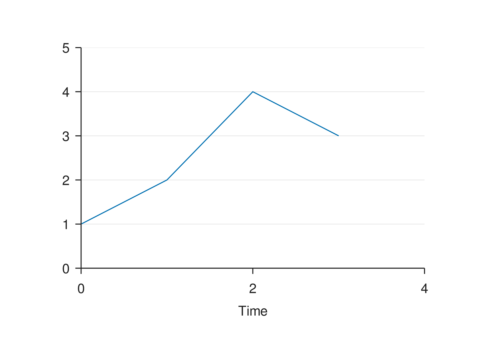
# Minimal complete example: axispage=canvas(size=(100mm,75mm),background="#ffffff")p=plot(size=(86mm,62mm),x=axis(range=(0,4),ticks=[0,2,4],label="Time"),y=axis(range=(0,5),grid=major))p.line(x=[0,1,2,3],y=[1,2,4,3])page.add(p,offset=(7mm,6mm))# Minimal complete example: axispage=canvas(size=(100mm,75mm),background="#ffffff")p=plot(size=(86mm,62mm),x=axis(range=(0,4),ticks=[0,2,4],label="Time"),y=axis(range=(0,5),grid=major))p.line(x=[0,1,2,3],y=[1,2,4,3])page.add(p,offset=(7mm,6mm))Preview
Dependencies
examples/manual/axis.lay
Parameters and default behavior#
Unitless geometry uses the canvas unit; unitless type and stroke sizes use pt. Explicit call parameters override inherited/theme defaults. The linked interface reference lists accepted types, choices and defaults per parameter.
Composition#
Use text or formula material in tick_text for independent formatting. tick_rotation rotates about each label center; a fixed plot_area helps compare the occupied space before and after rotation.
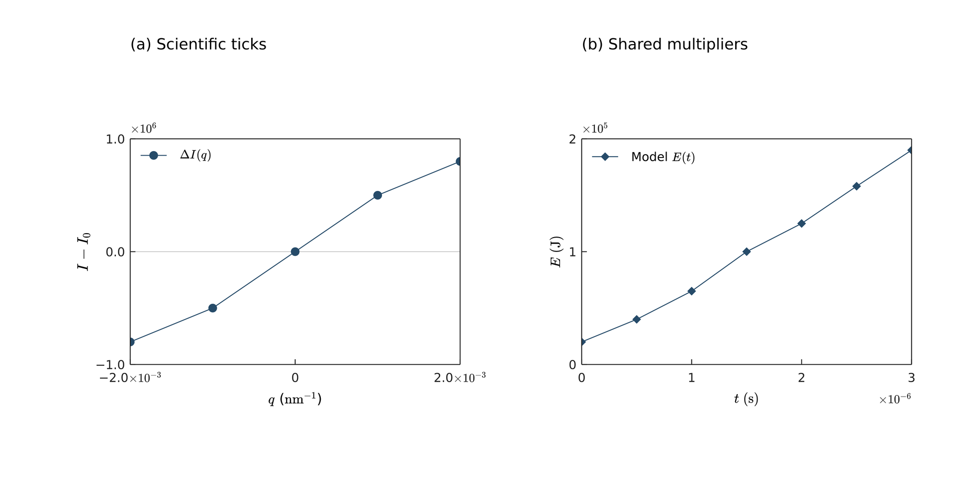
# Two independently placed 76 x 52 mm data rectangles.# Label and exponent offsets are independent chart-local physical lengths (right/down).# The short x title shares the multiplier row; only default collisions add a title row.page = canvas(size=(220 mm, 115 mm), background="#ffffff")style = plot_style(font_family="DejaVu Sans", font_size=8 pt, colors=["#264b69"])q_label = text(spans=[formula(source=r"q", font_size=9 pt), span(" ("), formula(source=r"\mathrm{nm}^{-1}", font_size=9 pt), span(")")], font_family="DejaVu Sans", font_size=9 pt)left = plot(size=(110 mm, 98 mm), plot_area=box(offset=(24 mm, 22 mm), size=(76 mm, 52 mm)), frame= box, style=style, x=axis(label=q_label, range=(-0.002, 0.002), ticks=[-0.002, 0, 0.002], notation= scientific, format=".1e", tick_direction= in), y=axis(label=formula(source=r"I-I_0", font_size=10 pt), range=(-1000000, 1000000), ticks=[-1000000, 0, 1000000], notation= offset, format=".1f", tick_direction= in))left.hline(y=0, color="#bbbbbb", line_width=0.4 pt)# Two independently placed 76 x 52 mm data rectangles.# Label and exponent offsets are independent chart-local physical lengths (right/down).# The short x title shares the multiplier row; only default collisions add a title row.page = canvas(size=(220 mm, 115 mm), background="#ffffff")style = plot_style(font_family="DejaVu Sans", font_size=8 pt, colors=["#264b69"])q_label = text(spans=[formula(source=r"q", font_size=9 pt), span(" ("), formula(source=r"\mathrm{nm}^{-1}", font_size=9 pt), span(")")], font_family="DejaVu Sans", font_size=9 pt)left = plot(size=(110 mm, 98 mm), plot_area=box(offset=(24 mm, 22 mm), size=(76 mm, 52 mm)), frame= box, style=style, x=axis(label=q_label, range=(-0.002, 0.002), ticks=[-0.002, 0, 0.002], notation= scientific, format=".1e", tick_direction= in), y=axis(label=formula(source=r"I-I_0", font_size=10 pt), range=(-1000000, 1000000), ticks=[-1000000, 0, 1000000], notation= offset, format=".1f", tick_direction= in))left.hline(y=0, color="#bbbbbb", line_width=0.4 pt)left.line(x=[-0.002, -0.001, 0, 0.001, 0.002], y=[-800000, -500000, 0, 500000, 800000], marker= circle, marker_size=2 mm, label=formula(source=r"\Delta I(q)", font_size=8 pt))left.legend(position= top_left, background="none")a = page.add(left, anchor= plot_top_left, offset=(30 mm, 32 mm))page.add(text(content="(a) Scientific ticks", font_family="DejaVu Sans", font_size=10 pt), target=a.plot_top_left, offset=(0 mm, -24 mm)) right = plot(size=(110 mm, 98 mm), plot_area=box(offset=(24 mm, 22 mm), size=(76 mm, 52 mm)), frame= box, style=style, x=axis(label=formula(source=r"t\;(\mathrm{s})", font_size=9 pt), range=(0, 0.000003), ticks=[0, 0.000001, 0.000002, 0.000003], notation= offset, exponent=-6, format=".0f", exponent_offset=(0 mm, -0.5 mm), label_offset=(0 mm, 0.5 mm), tick_direction= in), y=axis(label=formula(source=r"E\;(\mathrm{J})", font_size=9 pt), range=(0, 200000), ticks=[0, 100000, 200000], notation= offset, format=".0f", tick_direction= in))right.line(x=[0, 0.0000005, 0.000001, 0.0000015, 0.000002, 0.0000025, 0.000003], y=[20000, 40000, 65000, 100000, 125000, 158000, 190000], marker= diamond, marker_size=2 mm, label=text(spans=[span("Model "), formula(source=r"E(t)", font_size=8 pt)], font_family="DejaVu Sans", font_size=8 pt))right.legend(position= top_left, background="none")b = page.add(right, anchor= plot_top_left, offset=(134 mm, 32 mm))page.add(text(content="(b) Shared multipliers", font_family="DejaVu Sans", font_size=10 pt), target=b.plot_top_left, offset=(0 mm, -24 mm))Preview
Dependencies
examples/plot/scientific-labels.lay
Common errors and limits#
Explicit text/formula styles remain intact rather than being fully replaced by axis defaults. Do not multiply a displayed scientific factor into the input again. Layout warnings indicate insufficient label space.
Individual functions#
Detailed behavior and further examples#
Parameters#
| Parameter | Purpose | Default or requirement |
|---|---|---|
label |
Axis or legend label | String, text or formula |
tick_text |
Custom tick labels | Same length as ticks |
Common usage#
Axis, layer legend, and colorbar label values accept strings, text(...), or formula(...). Strings inherit the plot color and the relevant font size. Text/formula materials retain their own styling, explicit sizes, widths, and wrapping, without automatic scaling. Use existing text(spans=[...]) for mixed content. Relative font paths still resolve against the material's defining .lay file.
Axes and colorbar(...) share these options:
| Option | Display rule |
|---|---|
notation="plain" |
Default, retaining existing number formatting. format=".2e" still produces ordinary 1.00e+6 text |
notation="scientific" |
Each nonzero tick becomes a×10ⁿ with a mathematical superscript. Default precision is .2e; explicit format must have exponential type e. Zero displays as 0; rounding carries into the exponent |
notation="offset" |
One shared ×10ⁿ multiplier. The default exponent is the decimal order of the maximum absolute domain endpoint. A zero exponent omits the multiplier |
exponent=6 |
Explicit integer exponent, only for offset. Representable multipliers support -323…308; overflowing scaled ticks raise an error |
format=".1f" |
In offset mode formats the value divided by the multiplier; 1500000 with exponent 6 becomes 1.5 |
exponent_offset=(dx,dy) |
Only for offset; physical displacement, default (0 mm,0 mm). Positive x goes right, positive y goes down; negatives are allowed |
The x-axis multiplier sits below the ticks at the right; the y-axis multiplier sits above the axis at the left. tick_labels=false hides the multiplier too. Measured labels and multipliers contribute to surrounding space requirements. Notation changes only display: data and chart.data(...) use original values, with unchanged linear/log mappings. Insufficient fixed margins or plot_area space produce warnings while retaining the data rectangle and all manually placed neighboring panels.
The centered x-axis title normally shares the row below the ticks with the right-aligned multiplier. Only an overlap between their measured default bounds places the title below the multiplier, separated by 1.2 mm. Formula superscripts/subscripts, text widths and line breaks participate in measurement. Without an x-axis multiplier, the previous default title placement is retained.
axis(label_offset=(dx,dy)) shifts the title independently; exponent_offset shifts the multiplier independently. Offsets are applied after default placement and collision handling, so moving either decoration does not reposition the other. Both use chart-local physical coordinates, with x right and y down, followed by chart rotation or containing-group scaling. Even the rotated y-axis title translates along those two local directions. Offset-induced title/multiplier overlaps and insufficient space produce W_PLOT_LAYOUT while retaining the requested settings. Automatic margins measure required space; a legacy title positioned at the frame edge can still be shifted outside that frame, in which case its position is retained with a warning. Use plot_area to reserve explicit surrounding space. Colorbars also accept independent label_offset, retaining their existing layout rules.
For more complex title layouts, use independent page.add(text(...)) or group.add(text(...)) placements targeting data-rectangle anchors.
Editable source · SVG · PDF. Both data rectangles are explicitly 76 × 52 mm, with page top-left positions (30,32) mm and (134,32) mm. The right panel shifts its x-axis title down 0.5 mm and its multiplier up 0.5 mm while preserving the data rectangle.
Limits and related topics#
Data input and missing values · Plot area and physical size · Axes and ticks · Legends and shared colorbars · Data anchors and annotations