Heatmaps and contours#

Purpose and concepts#

heatmap represents cell values, contour represents sampled-field isolines and contourf fills level intervals. All require rectangular matrices, but cell edges differ from sample coordinates.

Minimal complete example#

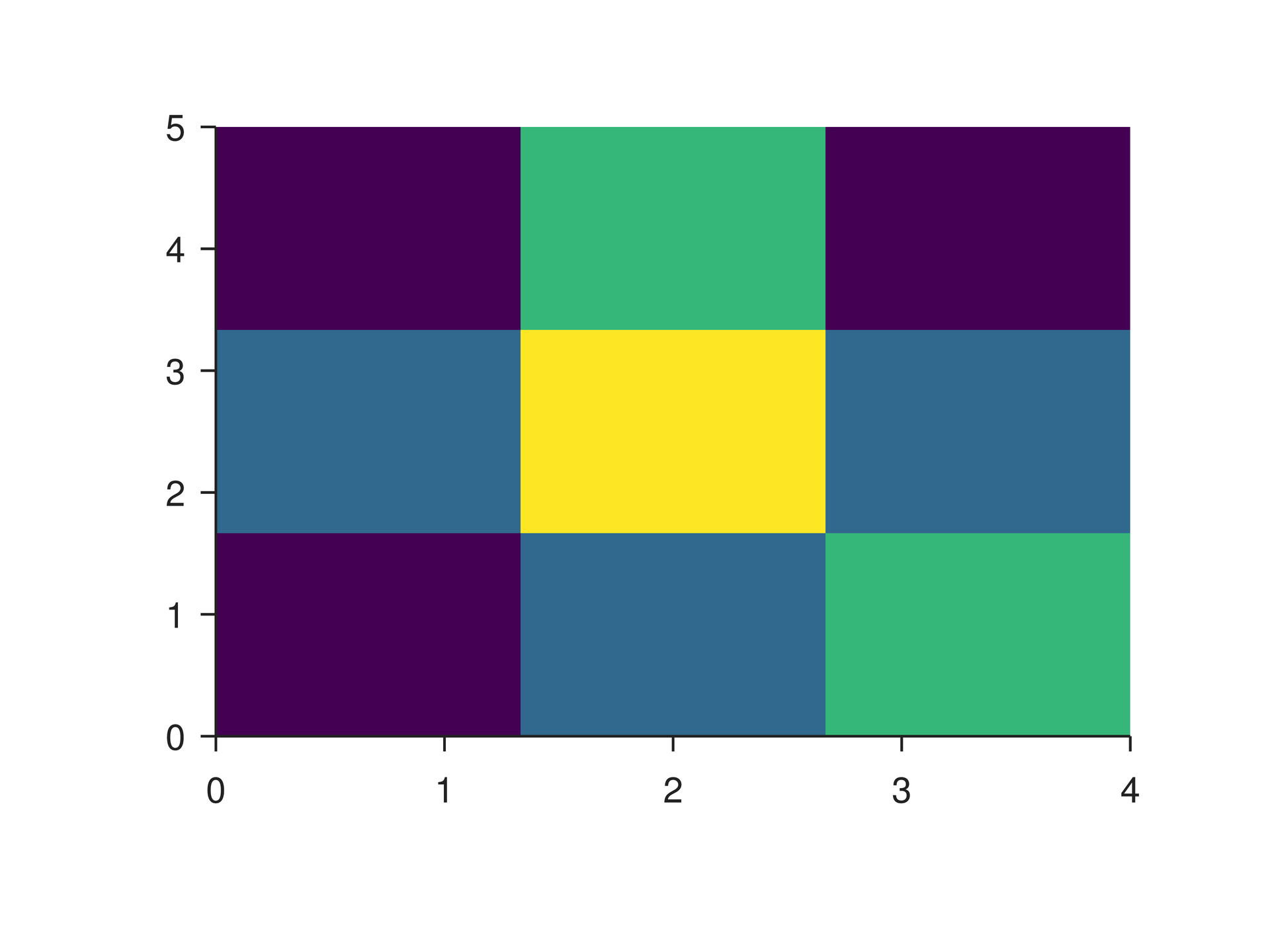
Run this file directly with laymesh validate or laymesh render; it contains its own canvas and required definitions.

1# Minimal complete example: plot.heatmap2page=canvas(size=(100mm,75mm),background="#ffffff")3p=plot(size=(86mm,62mm),x=axis(range=(0,4)),y=axis(range=(0,5)))4p.heatmap(z=[[1,2,3],[2,4,2],[1,3,1]],extent=(0,4,0,5),origin=lower)5page.add(p,offset=(7mm,6mm))

# Minimal complete example: plot.heatmap
page=canvas(size=(100mm,75mm),background="#ffffff")
p=plot(size=(86mm,62mm),x=axis(range=(0,4)),y=axis(range=(0,5)))
p.heatmap(z=[[1,2,3],[2,4,2],[1,3,1]],extent=(0,4,0,5),origin=lower)
page.add(p,offset=(7mm,6mm))

1# Minimal complete example: plot.heatmap2page=canvas(size=(100mm,75mm),background="#ffffff")3p=plot(size=(86mm,62mm),x=axis(range=(0,4)),y=axis(range=(0,5)))4p.heatmap(z=[[1,2,3],[2,4,2],[1,3,1]],extent=(0,4,0,5),origin=lower)5page.add(p,offset=(7mm,6mm))

# Minimal complete example: plot.heatmap
page=canvas(size=(100mm,75mm),background="#ffffff")
p=plot(size=(86mm,62mm),x=axis(range=(0,4)),y=axis(range=(0,5)))
p.heatmap(z=[[1,2,3],[2,4,2],[1,3,1]],extent=(0,4,0,5),origin=lower)
page.add(p,offset=(7mm,6mm))

Dependencies

examples/manual/plot-heatmap.lay

Parameters and default behavior#

Unitless geometry uses the canvas unit; unitless type and stroke sizes use pt. Explicit call parameters override inherited/theme defaults. The linked interface reference lists accepted types, choices and defaults per parameter.

Composition#

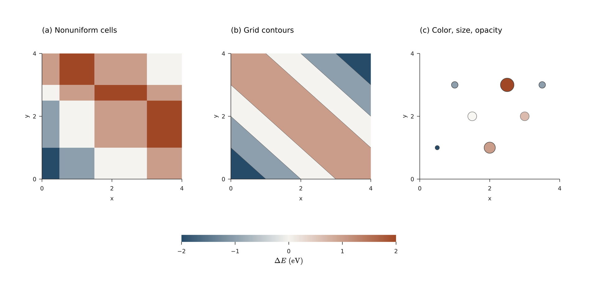
Share color_scale across heatmaps and contours. x_edges/y_edges are heatmap boundaries; contour x/y are sample coordinates. Nonuniform or broken axes use vector cells for accurate mapping.

2# One physical color scale for nonuniform cells, contours and point colors.3page=canvas(size=(256 mm,132 mm),background="#ffffff")4s=plot_style(font_family="DejaVu Sans",font_size=7 pt)5colors=color_scale(norm= centered,vmin=-2,vmax=2,center=0,cmap=["#264b69","#f4f3ef","#a04725"])6a=plot(size=(82 mm,92 mm),plot_area=box(offset=(16 mm, 18 mm), size=(60 mm, 54 mm)),style=s,x=axis(label="x",range=(0,4),ticks=[0,2,4]),y=axis(label="y",range=(0,4),ticks=[0,2,4]))7a.heatmap(z=[[-2,-1,0,1],[-1,0,1,2],[0,1,2,1],[1,2,1,0]],x_edges=[0,0.5,1.5,3,4],y_edges=[0,1,2.5,3,4],color_scale=colors)8ca=page.add(a,offset=(2 mm,5 mm))9page.add(text(content="(a) Nonuniform cells",font_family="DejaVu Sans",font_size=9 pt),target=ca.plot_top_left,offset=(0 mm,-12 mm))10b=plot(size=(82 mm,92 mm),plot_area=box(offset=(16 mm, 18 mm), size=(60 mm, 54 mm)),style=s,x=axis(label="x",range=(0,4),ticks=[0,2,4]),y=axis(label="y",range=(0,4),ticks=[0,2,4]))11b.contourf(z=[[-2,-1,0,1,2],[-1,0,1,2,1],[0,1,2,1,0],[1,2,1,0,-1],[2,1,0,-1,-2]],x=[0,1,2,3,4],y=[0,1,2,3,4],levels=[-2,-1,0,1],color_scale=colors)12b.contour(z=[[-2,-1,0,1,2],[-1,0,1,2,1],[0,1,2,1,0],[1,2,1,0,-1],[2,1,0,-1,-2]],levels=[-1,0,1],color="#555555",line_width=0.3 pt)13cb=page.add(b,offset=(83 mm,5 mm))14page.add(text(content="(b) Grid contours",font_family="DejaVu Sans",font_size=9 pt),target=cb.plot_top_left,offset=(0 mm,-12 mm))15c=plot(size=(82 mm,92 mm),plot_area=box(offset=(16 mm, 18 mm), size=(60 mm, 54 mm)),style=s,x=axis(label="x",range=(0,4),ticks=[0,2,4]),y=axis(label="y",range=(0,4),ticks=[0,2,4]))16c.scatter(x=[0.5,1,1.5,2,2.5,3,3.5],y=[1,3,2,1,3,2,3],c=[-2,-1,0,1,2,1,-1],color_scale=colors,marker_size=[2 mm,3 mm,4 mm,5 mm,6 mm,4 mm,3 mm],opacity=[1,1,0.7,1,1,0.7,1],marker_border_color="#444444",marker_border_width=0.2 mm)17cc=page.add(c,offset=(164 mm,5 mm))18page.add(text(content="(c) Color, size, opacity",font_family="DejaVu Sans",font_size=9 pt),target=cc.plot_top_left,offset=(0 mm,-12 mm))19page.add(colorbar(scale=colors,orientation= horizontal,length=92 mm,ticks=[-2,-1,0,1,2],label=formula(source=r"\Delta E\;(\mathrm{eV})",font_size=9 pt),style=s),offset=(76 mm,101 mm))

# One physical color scale for nonuniform cells, contours and point colors.
page=canvas(size=(256 mm,132 mm),background="#ffffff")
s=plot_style(font_family="DejaVu Sans",font_size=7 pt)
colors=color_scale(norm= centered,vmin=-2,vmax=2,center=0,cmap=["#264b69","#f4f3ef","#a04725"])
a=plot(size=(82 mm,92 mm),plot_area=box(offset=(16 mm, 18 mm), size=(60 mm, 54 mm)),style=s,x=axis(label="x",range=(0,4),ticks=[0,2,4]),y=axis(label="y",range=(0,4),ticks=[0,2,4]))
a.heatmap(z=[[-2,-1,0,1],[-1,0,1,2],[0,1,2,1],[1,2,1,0]],x_edges=[0,0.5,1.5,3,4],y_edges=[0,1,2.5,3,4],color_scale=colors)
ca=page.add(a,offset=(2 mm,5 mm))
page.add(text(content="(a) Nonuniform cells",font_family="DejaVu Sans",font_size=9 pt),target=ca.plot_top_left,offset=(0 mm,-12 mm))
b=plot(size=(82 mm,92 mm),plot_area=box(offset=(16 mm, 18 mm), size=(60 mm, 54 mm)),style=s,x=axis(label="x",range=(0,4),ticks=[0,2,4]),y=axis(label="y",range=(0,4),ticks=[0,2,4]))
b.contourf(z=[[-2,-1,0,1,2],[-1,0,1,2,1],[0,1,2,1,0],[1,2,1,0,-1],[2,1,0,-1,-2]],x=[0,1,2,3,4],y=[0,1,2,3,4],levels=[-2,-1,0,1],color_scale=colors)
b.contour(z=[[-2,-1,0,1,2],[-1,0,1,2,1],[0,1,2,1,0],[1,2,1,0,-1],[2,1,0,-1,-2]],levels=[-1,0,1],color="#555555",line_width=0.3 pt)
cb=page.add(b,offset=(83 mm,5 mm))
page.add(text(content="(b) Grid contours",font_family="DejaVu Sans",font_size=9 pt),target=cb.plot_top_left,offset=(0 mm,-12 mm))
c=plot(size=(82 mm,92 mm),plot_area=box(offset=(16 mm, 18 mm), size=(60 mm, 54 mm)),style=s,x=axis(label="x",range=(0,4),ticks=[0,2,4]),y=axis(label="y",range=(0,4),ticks=[0,2,4]))
c.scatter(x=[0.5,1,1.5,2,2.5,3,3.5],y=[1,3,2,1,3,2,3],c=[-2,-1,0,1,2,1,-1],color_scale=colors,marker_size=[2 mm,3 mm,4 mm,5 mm,6 mm,4 mm,3 mm],opacity=[1,1,0.7,1,1,0.7,1],marker_border_color="#444444",marker_border_width=0.2 mm)
cc=page.add(c,offset=(164 mm,5 mm))
page.add(text(content="(c) Color, size, opacity",font_family="DejaVu Sans",font_size=9 pt),target=cc.plot_top_left,offset=(0 mm,-12 mm))
page.add(colorbar(scale=colors,orientation= horizontal,length=92 mm,ticks=[-2,-1,0,1,2],label=formula(source=r"\Delta E\;(\mathrm{eV})",font_size=9 pt),style=s),offset=(76 mm,101 mm))

1# BEGIN DEMO2# One physical color scale for nonuniform cells, contours and point colors.3page=canvas(size=(256 mm,132 mm),background="#ffffff")4s=plot_style(font_family="DejaVu Sans",font_size=7 pt)5colors=color_scale(norm= centered,vmin=-2,vmax=2,center=0,cmap=["#264b69","#f4f3ef","#a04725"])6a=plot(size=(82 mm,92 mm),plot_area=box(offset=(16 mm, 18 mm), size=(60 mm, 54 mm)),style=s,x=axis(label="x",range=(0,4),ticks=[0,2,4]),y=axis(label="y",range=(0,4),ticks=[0,2,4]))7a.heatmap(z=[[-2,-1,0,1],[-1,0,1,2],[0,1,2,1],[1,2,1,0]],x_edges=[0,0.5,1.5,3,4],y_edges=[0,1,2.5,3,4],color_scale=colors)8ca=page.add(a,offset=(2 mm,5 mm))9page.add(text(content="(a) Nonuniform cells",font_family="DejaVu Sans",font_size=9 pt),target=ca.plot_top_left,offset=(0 mm,-12 mm))10b=plot(size=(82 mm,92 mm),plot_area=box(offset=(16 mm, 18 mm), size=(60 mm, 54 mm)),style=s,x=axis(label="x",range=(0,4),ticks=[0,2,4]),y=axis(label="y",range=(0,4),ticks=[0,2,4]))11b.contourf(z=[[-2,-1,0,1,2],[-1,0,1,2,1],[0,1,2,1,0],[1,2,1,0,-1],[2,1,0,-1,-2]],x=[0,1,2,3,4],y=[0,1,2,3,4],levels=[-2,-1,0,1],color_scale=colors)12b.contour(z=[[-2,-1,0,1,2],[-1,0,1,2,1],[0,1,2,1,0],[1,2,1,0,-1],[2,1,0,-1,-2]],levels=[-1,0,1],color="#555555",line_width=0.3 pt)13cb=page.add(b,offset=(83 mm,5 mm))14page.add(text(content="(b) Grid contours",font_family="DejaVu Sans",font_size=9 pt),target=cb.plot_top_left,offset=(0 mm,-12 mm))15c=plot(size=(82 mm,92 mm),plot_area=box(offset=(16 mm, 18 mm), size=(60 mm, 54 mm)),style=s,x=axis(label="x",range=(0,4),ticks=[0,2,4]),y=axis(label="y",range=(0,4),ticks=[0,2,4]))16c.scatter(x=[0.5,1,1.5,2,2.5,3,3.5],y=[1,3,2,1,3,2,3],c=[-2,-1,0,1,2,1,-1],color_scale=colors,marker_size=[2 mm,3 mm,4 mm,5 mm,6 mm,4 mm,3 mm],opacity=[1,1,0.7,1,1,0.7,1],marker_border_color="#444444",marker_border_width=0.2 mm)17cc=page.add(c,offset=(164 mm,5 mm))18page.add(text(content="(c) Color, size, opacity",font_family="DejaVu Sans",font_size=9 pt),target=cc.plot_top_left,offset=(0 mm,-12 mm))19page.add(colorbar(scale=colors,orientation= horizontal,length=92 mm,ticks=[-2,-1,0,1,2],label=formula(source=r"\Delta E\;(\mathrm{eV})",font_size=9 pt),style=s),offset=(76 mm,101 mm))20# END DEMO

# BEGIN DEMO
# One physical color scale for nonuniform cells, contours and point colors.
page=canvas(size=(256 mm,132 mm),background="#ffffff")
s=plot_style(font_family="DejaVu Sans",font_size=7 pt)
colors=color_scale(norm= centered,vmin=-2,vmax=2,center=0,cmap=["#264b69","#f4f3ef","#a04725"])
a=plot(size=(82 mm,92 mm),plot_area=box(offset=(16 mm, 18 mm), size=(60 mm, 54 mm)),style=s,x=axis(label="x",range=(0,4),ticks=[0,2,4]),y=axis(label="y",range=(0,4),ticks=[0,2,4]))
a.heatmap(z=[[-2,-1,0,1],[-1,0,1,2],[0,1,2,1],[1,2,1,0]],x_edges=[0,0.5,1.5,3,4],y_edges=[0,1,2.5,3,4],color_scale=colors)
ca=page.add(a,offset=(2 mm,5 mm))
page.add(text(content="(a) Nonuniform cells",font_family="DejaVu Sans",font_size=9 pt),target=ca.plot_top_left,offset=(0 mm,-12 mm))
b=plot(size=(82 mm,92 mm),plot_area=box(offset=(16 mm, 18 mm), size=(60 mm, 54 mm)),style=s,x=axis(label="x",range=(0,4),ticks=[0,2,4]),y=axis(label="y",range=(0,4),ticks=[0,2,4]))
b.contourf(z=[[-2,-1,0,1,2],[-1,0,1,2,1],[0,1,2,1,0],[1,2,1,0,-1],[2,1,0,-1,-2]],x=[0,1,2,3,4],y=[0,1,2,3,4],levels=[-2,-1,0,1],color_scale=colors)
b.contour(z=[[-2,-1,0,1,2],[-1,0,1,2,1],[0,1,2,1,0],[1,2,1,0,-1],[2,1,0,-1,-2]],levels=[-1,0,1],color="#555555",line_width=0.3 pt)
cb=page.add(b,offset=(83 mm,5 mm))
page.add(text(content="(b) Grid contours",font_family="DejaVu Sans",font_size=9 pt),target=cb.plot_top_left,offset=(0 mm,-12 mm))
c=plot(size=(82 mm,92 mm),plot_area=box(offset=(16 mm, 18 mm), size=(60 mm, 54 mm)),style=s,x=axis(label="x",range=(0,4),ticks=[0,2,4]),y=axis(label="y",range=(0,4),ticks=[0,2,4]))
c.scatter(x=[0.5,1,1.5,2,2.5,3,3.5],y=[1,3,2,1,3,2,3],c=[-2,-1,0,1,2,1,-1],color_scale=colors,marker_size=[2 mm,3 mm,4 mm,5 mm,6 mm,4 mm,3 mm],opacity=[1,1,0.7,1,1,0.7,1],marker_border_color="#444444",marker_border_width=0.2 mm)
cc=page.add(c,offset=(164 mm,5 mm))
page.add(text(content="(c) Color, size, opacity",font_family="DejaVu Sans",font_size=9 pt),target=cc.plot_top_left,offset=(0 mm,-12 mm))
page.add(colorbar(scale=colors,orientation= horizontal,length=92 mm,ticks=[-2,-1,0,1,2],label=formula(source=r"\Delta E\;(\mathrm{eV})",font_size=9 pt),style=s),offset=(76 mm,101 mm))
# END DEMO

Dependencies

examples/plot/shared-colors.lay

Common errors and limits#

levels must increase and contours need at least 2×2 samples. Missing regions are not interpolated and scattered observations do not become a grid automatically. Coordinates and extent are exclusive; ragged rows error.

Individual functions#

plot-heatmap#

Heatmap layer: add data to this plot, control its appearance with physical style parameters, and select data mappings with named-axis parameters.

Returns: A layer handle that can be included in a shared legend.

Minimal complete source · Composition source · All parameters

plot-contour#

Contours layer: add data to this plot, control its appearance with physical style parameters, and select data mappings with named-axis parameters.

Returns: A layer handle that can be included in a shared legend.

Minimal complete source · Composition source · All parameters

plot-contourf#

Filled contours layer: add data to this plot, control its appearance with physical style parameters, and select data mappings with named-axis parameters.

Returns: A layer handle that can be included in a shared legend.

Minimal complete source · Composition source · All parameters

Detailed behavior and further examples#

Parameters#

Parameter	Purpose	Default or requirement
`z`	2D data matrix	Equal-length rows
`x_edges / y_edges`	Cell edges	Strictly increasing; exclusive with extent
`levels`	Contour levels	Strictly increasing

Common usage#

Continuous norms linear/log/symlog/centered require explicit finite increasing vmin/vmax. Log requires positive bounds and valid data. Symlog accepts positive constant; centered requires center strictly inside the range. Discrete scales use norm="boundary",boundaries=[...] instead of vmin/vmax. An internal boundary belongs to the interval on its right; the maximum belongs to the last interval.

cmap accepts all Matplotlib 3.11.2 presets, an immutable cmap(...) handle, or at least two custom colors. Continuous sequences interpolate linearly in RGB; discrete sequences select interval colors. Missing data is transparent. Outside values clamp by default, with optional under/over colors. Heatmaps, points, contours and colorbars reuse the exact mapping. Legacy heatmap cmap/vmin/vmax retain a private linear mapping; combining them with color_scale errors.

Scatter c and marker_fill are mutually exclusive. c must match x/y length. marker_size accepts a matching list of physical lengths, opacity a matching array in 0–1. Each stroke stays within its marker's final outer box. Legends use the layer's scalar default sample for per-point size/opacity; a colorbar explains numerical point colors.

Heatmap x_edges/y_edges are increasing cell boundaries, with columns+1/rows+1 entries. They conflict with extent; an unspecified dimension retains default uniform boundaries. Nonlinear axes, broken axes and nonuniform cells use vector cell geometry for accurate mapping. Original uniform linear heatmaps retain their default raster path.

contour/contourf require at least a 2×2 rectangular matrix and explicit increasing levels. x/y specify grid sample coordinates; defaults are 0..columns-1/0..rows-1, or sample endpoints from extent. x/y and extent are mutually exclusive. D3 contour coordinates (i+0.5,j+0.5) are corrected to actual samples, including nonuniform spacing. Cells adjacent to missing samples remain empty; scattered points are never interpolated automatically.

Filled levels define interval lower bounds: regions below the first are empty, the highest extends upward. Subtracting adjacent nested superlevel sets produces disjoint bands, preserving translucent opacity. Without a scale, contourf creates a private viridis mapping from finite data, while contour uses the layer's single color.

Lines and scatter · Error bars and bands · Bars and steps · Multiple axes and breaks

Heatmaps and contours#

Purpose and concepts#

Minimal complete example#

Parameters and default behavior#

Composition#

Common errors and limits#

Individual functions#

plot-heatmap#

plot-contour#

plot-contourf#

Detailed behavior and further examples#

Parameters#

Common usage#

Limits and related topics#