 LayMesh
Scientific data plots#
Cartesian, polar and radar plots with fixed physical data areas and manually placed panels and decorations.
Back to the gallery · Execution results
Precise coordinates and statistics#
Multiple axes and independent gaps#
Three vertical axes have different breaks and physical gaps; the horizontal axis is independently broken. Edit the fixed data rectangle and axis offsets directly.
# Independent axis gaps. Lengths are literal mm, not stretch factors.page=canvas(size=(210 mm,128 mm),background="#ffffff")s=plot_style(font_family="DejaVu Sans",font_size=8 pt)p=plot(size=(195 mm,112 mm),plot_area=box(offset=(24 mm, 20 mm), size=(110 mm, 62 mm)),style=s, x=axis(label="Time (s)",range=(0,10),ticks=[0,1,2,8,9,10],breaks=[(2,8)],break_gap=3 mm,segment_lengths=[45 mm,62 mm],minor_ticks="auto"), y=axis(label="Signal (a.u.)",range=(0,100),ticks=[0,5,80,90,100],breaks=[(10,80)],break_gap=2 mm,segment_lengths=[20 mm,40 mm],line_color="#264b69"))p.add_axis(name="temperature",side="right",offset=0 mm, axis=axis(label="Temperature (K)",range=(200,1000),ticks=[200,400,800,1000],breaks=[(400,800)],break_gap=4 mm,segment_lengths=[29 mm,29 mm],line_color="#a04725"))p.add_axis(name="pressure",side="right",offset=29 mm, axis=axis(label="Pressure (MPa)",range=(0,100),ticks=[0,25,50,75,100],line_color="#34705a"))a=p.line(x=[0,1,2,8,9,10],y=[1,5,9,84,92,98],marker="circle",color="#264b69",label="Signal")b=p.line(x=[0,1,2,8,9,10],y=[220,300,380,830,910,980],y_axis="temperature",marker="diamond",color="#a04725",label="Temperature")c=p.line(x=[0,1,2,8,9,10],y=[15,26,40,55,72,91],y_axis="pressure",line_dash=[2 mm,1 mm],color="#34705a",label="Pressure")p.errorbar(x=[1,9],y=[5,91],yerr=[4,8],color="#264b69",cap_size=2 mm)chart=page.add(p,offset=(6 mm,8 mm))page.add(text(content="Independent gaps on three vertical axes",font_family="DejaVu Sans",font_size=10 pt),target=chart.plot_top_left,offset=(0 mm,-14 mm))page.add(legend(layers=[a,b,c],columns=3,gap=3 mm,background="none"),target=chart.plot_bottom_left,offset=(0 mm,23 mm))# This data anchor uses temperature values, including its independent break.page.add(text(content="T",font_family="DejaVu Sans",font_size=8 pt,color="#a04725"),anchor=bottom_left,target=chart.data(x=9,y=910,y_axis="temperature"),offset=(2 mm,-2 mm))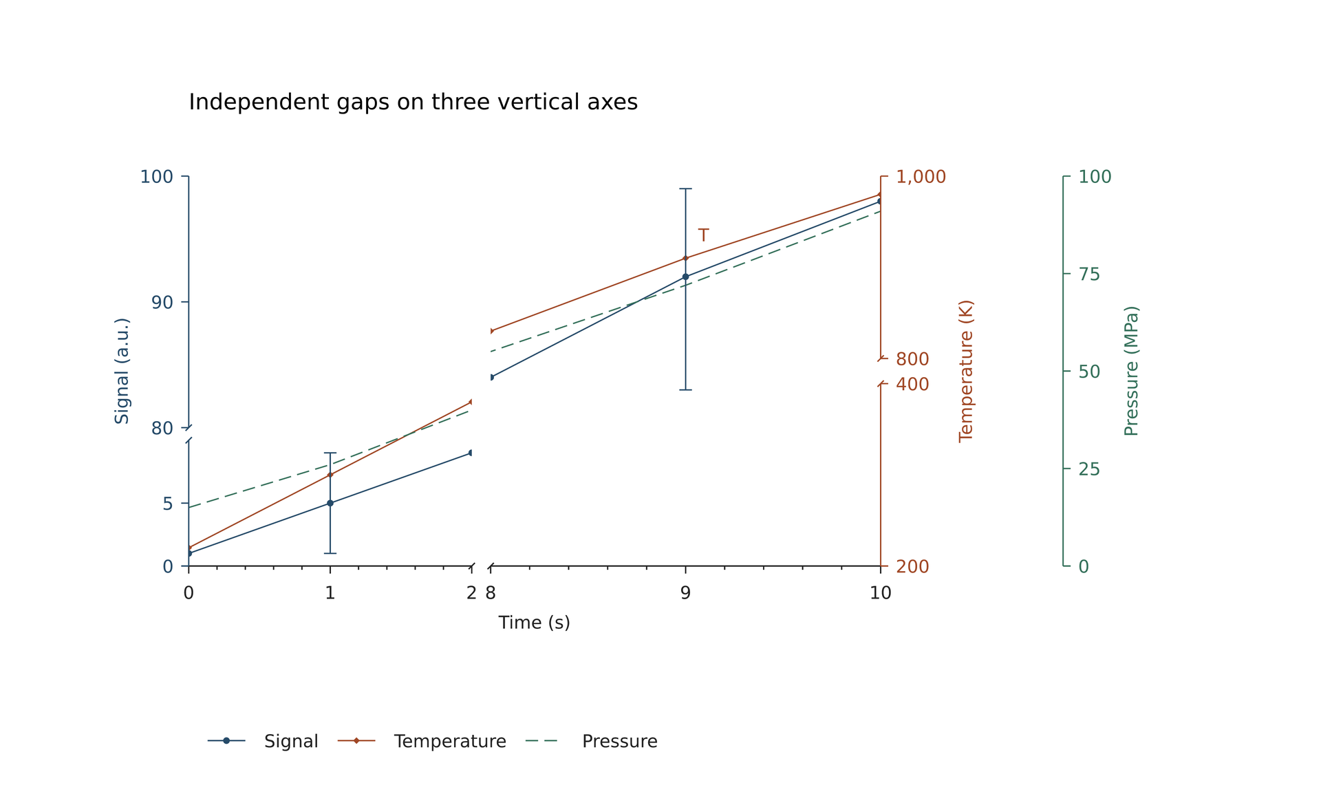
Source: multi-axes-breaks.lay.
Reproduce: laymesh validate examples/plot/multi-axes-breaks.lay; laymesh render examples/plot/multi-axes-breaks.lay -o multi-axes-breaks.png --dpi 150.
Observed CLI output: 有效:examples/plot/multi-axes-breaks.lay(210 × 128 mm,4 个顶层实例); PNG 1240 × 756 px at 150 DPI; warnings: none.
Layers and descriptive statistics#
Explicit bar positions and stacking baselines, steps, histogram density, ECDF, boxes and violins. A constant violin sample intentionally shows its median and warns.
# Statistics are evaluated in original data units. Positions preserve input order.page=canvas(size=(274 mm,128 mm),background="#ffffff")s=plot_style(font_family="DejaVu Sans",font_size=7 pt)a=plot(size=(88 mm,91 mm),plot_area=box(offset=(16 mm, 15 mm), size=(62 mm, 55 mm)),style=s, x=axis(range=(0,5),ticks=[1,2,3,4],tick_text=["A","B","C","D"]),y=axis(label="Change",range=(-2,7),ticks=[-2,0,2,4,6]))bar=a.bar(positions=[1,2,3,4],values=[2,-1,4,3],data_width=0.65,fill="#e0e6eb",border_color="#264b69",hatch="slash",hatch_spacing=1.5 mm,label="Change")a.bar(positions=[1,3,4],values=[1,1,2],baseline=[2,4,3],data_width=0.65,fill="none",border_color="#a04725",hatch="cross",label="Stack")a.hline(y=0,color="#777777",line_width=0.3 pt)a.step(x=[0.5,1.5,2.5,3.5,4.5],y=[1,2,1,3,4],where="post",color="#a04725")ca=page.add(a,offset=(4 mm,10 mm))page.add(text(content="(a) Bars, stacks and steps",font_family="DejaVu Sans",font_size=9 pt),target=ca.plot_top_left,offset=(0 mm,-12 mm)) b=plot(size=(104 mm,91 mm),plot_area=box(offset=(16 mm, 15 mm), size=(62 mm, 55 mm)),style=s, x=axis(label="Observation",range=(0,6),ticks=[0,2,4,6]),y=axis(label="Density",range=(0,0.5),ticks=[0,0.2,0.4]))b.add_axis(name="cumulative",side="right",axis=axis(label="ECDF",range=(0,1),ticks=[0,0.5,1],line_color="#a04725"))hist=b.hist(values=[0.4,0.8,1.1,1.2,1.6,2.2,2.3,2.8,3.1,3.8,4.1,5.4],bins=[0,1,2,3,4,6],stat="density",fill="#d9e5dd",border_color="#34705a",label="Density")ecdf=b.ecdf(values=[0.4,0.8,1.1,1.2,1.6,2.2,2.3,2.8,3.1,3.8,4.1,5.4],y_axis="cumulative",color="#a04725",label="ECDF")cb=page.add(b,offset=(90 mm,10 mm))page.add(text(content="(b) Histogram and ECDF",font_family="DejaVu Sans",font_size=9 pt),target=cb.plot_top_left,offset=(0 mm,-12 mm)) c=plot(size=(88 mm,91 mm),plot_area=box(offset=(20 mm, 15 mm), size=(62 mm, 55 mm)),style=s, x=axis(range=(0,4),ticks=[1,2,3],tick_text=["Box","KDE","Constant"]),y=axis(label="Observation",range=(0,11),ticks=[0,5,10]))box=c.boxplot(values=[1,2,2,3,3,4,5,10],position=1,data_width=0.65,fill="#e0e6eb",border_color="#264b69",label="R-7 / 1.5 IQR")violin=c.violin(values=[1,1.5,2,2.2,2.4,3,3.5,4.8,5],position=2,data_width=0.75,fill="#e8d8d1",border_color="#a04725",label="Gaussian KDE")c.violin(values=[3,3,3],position=3,data_width=0.65,color="#34705a")cc=page.add(c,offset=(179 mm,10 mm))page.add(text(content="(c) Box and violin",font_family="DejaVu Sans",font_size=9 pt),target=cc.plot_top_left,offset=(0 mm,-12 mm))page.add(legend(layers=[bar,hist,ecdf,box,violin],columns=5,gap=3 mm,background="none",sample_width=5 mm,sample_gap=2 mm),offset=(25 mm,105 mm))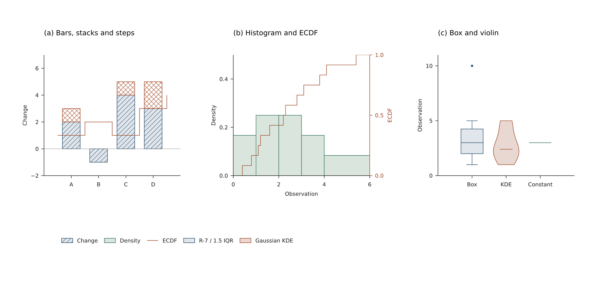
Source: statistics.lay.
Reproduce: laymesh validate examples/plot/statistics.lay; laymesh render examples/plot/statistics.lay -o statistics.png --dpi 150.
Observed CLI output: 有效:examples/plot/statistics.lay(274 × 128 mm,7 个顶层实例); PNG 1618 × 756 px at 150 DPI; warnings: examples/plot/statistics.lay:26:1: W_PLOT_MISSING: 样本不足或为常量,小提琴图仅显示中位数.
Shared colors and independent colorbar#
Nonuniform heatmap cells, grid contours and per-point color/size/opacity share one centered diverging scale. The standalone horizontal colorbar is positioned manually.
# One physical color scale for nonuniform cells, contours and point colors.page=canvas(size=(256 mm,132 mm),background="#ffffff")s=plot_style(font_family="DejaVu Sans",font_size=7 pt)colors=color_scale(norm="centered",vmin=-2,vmax=2,center=0,cmap=["#264b69","#f4f3ef","#a04725"])a=plot(size=(82 mm,92 mm),plot_area=box(offset=(16 mm, 18 mm), size=(60 mm, 54 mm)),style=s,x=axis(label="x",range=(0,4),ticks=[0,2,4]),y=axis(label="y",range=(0,4),ticks=[0,2,4]))a.heatmap(z=[[-2,-1,0,1],[-1,0,1,2],[0,1,2,1],[1,2,1,0]],x_edges=[0,0.5,1.5,3,4],y_edges=[0,1,2.5,3,4],color_scale=colors)ca=page.add(a,offset=(2 mm,5 mm))page.add(text(content="(a) Nonuniform cells",font_family="DejaVu Sans",font_size=9 pt),target=ca.plot_top_left,offset=(0 mm,-12 mm))b=plot(size=(82 mm,92 mm),plot_area=box(offset=(16 mm, 18 mm), size=(60 mm, 54 mm)),style=s,x=axis(label="x",range=(0,4),ticks=[0,2,4]),y=axis(label="y",range=(0,4),ticks=[0,2,4]))b.contourf(z=[[-2,-1,0,1,2],[-1,0,1,2,1],[0,1,2,1,0],[1,2,1,0,-1],[2,1,0,-1,-2]],x=[0,1,2,3,4],y=[0,1,2,3,4],levels=[-2,-1,0,1],color_scale=colors)b.contour(z=[[-2,-1,0,1,2],[-1,0,1,2,1],[0,1,2,1,0],[1,2,1,0,-1],[2,1,0,-1,-2]],levels=[-1,0,1],color="#555555",line_width=0.3 pt)cb=page.add(b,offset=(83 mm,5 mm))page.add(text(content="(b) Grid contours",font_family="DejaVu Sans",font_size=9 pt),target=cb.plot_top_left,offset=(0 mm,-12 mm))c=plot(size=(82 mm,92 mm),plot_area=box(offset=(16 mm, 18 mm), size=(60 mm, 54 mm)),style=s,x=axis(label="x",range=(0,4),ticks=[0,2,4]),y=axis(label="y",range=(0,4),ticks=[0,2,4]))c.scatter(x=[0.5,1,1.5,2,2.5,3,3.5],y=[1,3,2,1,3,2,3],c=[-2,-1,0,1,2,1,-1],color_scale=colors,marker_size=[2 mm,3 mm,4 mm,5 mm,6 mm,4 mm,3 mm],opacity=[1,1,0.7,1,1,0.7,1],marker_border_color="#444444",marker_border_width=0.2 mm)cc=page.add(c,offset=(164 mm,5 mm))page.add(text(content="(c) Color, size, opacity",font_family="DejaVu Sans",font_size=9 pt),target=cc.plot_top_left,offset=(0 mm,-12 mm))page.add(colorbar(scale=colors,orientation="horizontal",length=92 mm,ticks=[-2,-1,0,1,2],label=formula(source=r"\Delta E\;(\mathrm{eV})",font_size=9 pt),style=s),offset=(76 mm,101 mm))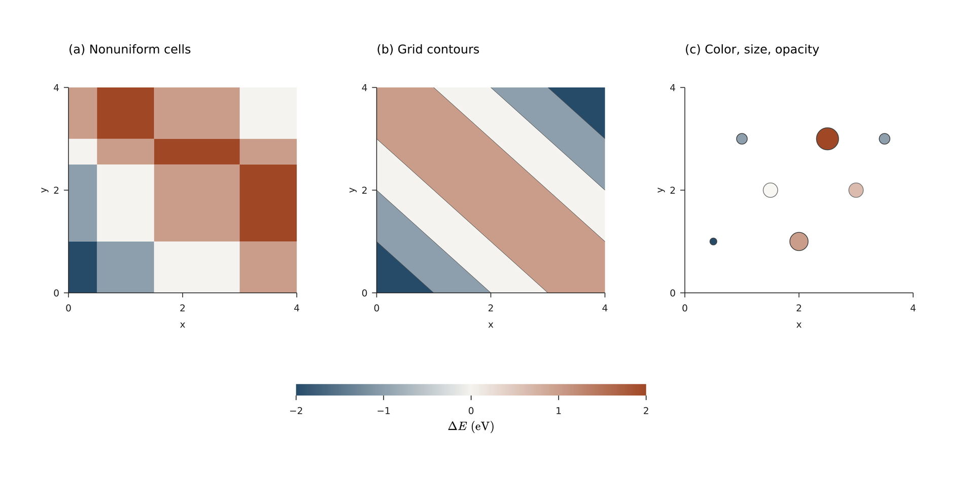
Source: shared-colors.lay.
Reproduce: laymesh validate examples/plot/shared-colors.lay; laymesh render examples/plot/shared-colors.lay -o shared-colors.png --dpi 150.
Observed CLI output: 有效:examples/plot/shared-colors.lay(256 × 132 mm,7 个顶层实例); PNG 1512 × 780 px at 150 DPI; warnings: none.
Manual inset#
Separate plots, an arrow and text are composed with existing anchors inside one group. The main symlog plot and the linear inset retain independent mappings.
# Insets are independent plots; placement stays completely manual and editable.page=canvas(size=(154 mm,112 mm),background="#ffffff")s=plot_style(font_family="DejaVu Sans",font_size=8 pt)p=plot(size=(140 mm,102 mm),plot_area=box(offset=(20 mm, 18 mm), size=(105 mm, 64 mm)),style=s,x=axis(label="Time (s)",range=(0,10)),y=axis(label="Response",scale="symlog",constant=0.5,range=(-1,100),ticks=[-1,0,1,10,100]))a=p.line(x=[0,1,2,3,4,5,6,7,8,9,10],y=[-0.5,0,0.4,1,2,4,8,16,32,64,90],marker="circle",color="#264b69",label="Observed")g=group()chart=g.add(p)# Add a white inset background as a separate editable shape.g.add(rect(size=(44 mm, 35 mm),fill="#ffffff",border_color="#bbbbbb",border_width=0.3 pt),target=chart.plot_top_left,offset=(4 mm,3 mm))zoom=plot(size=(44 mm,35 mm),plot_area=box(offset=(9 mm, 3 mm), size=(31 mm, 23 mm)),style=s,x=axis(range=(0,3),ticks=[0,1,2,3],tick_font_size=6 pt,tick_color="#555555"),y=axis(range=(-0.6,1.2),ticks=[0,1],tick_font_size=6 pt))zoom.line(x=[0,1,2,3],y=[-0.5,0,0.4,1],marker="circle",marker_size=1 mm,color="#264b69")inset=g.add(zoom,target=chart.plot_top_left,offset=(4 mm,3 mm))g.add(line(end_head=head(), dx=7 mm,dy=6 mm,line_color="#777777",line_width=0.4 pt),anchor="end",target=chart.data(x=3,y=1),offset=(0 mm,-1 mm))g.add(text(content="Local detail",font_family="DejaVu Sans",font_size=7 pt),target=inset.plot_top_left,offset=(0 mm,-6 mm))g.add(legend(layers=[a],background="none"),target=chart.plot_top_right,anchor=top_right,offset=(0 mm,-10 mm))page.add(g,offset=(6 mm,4 mm))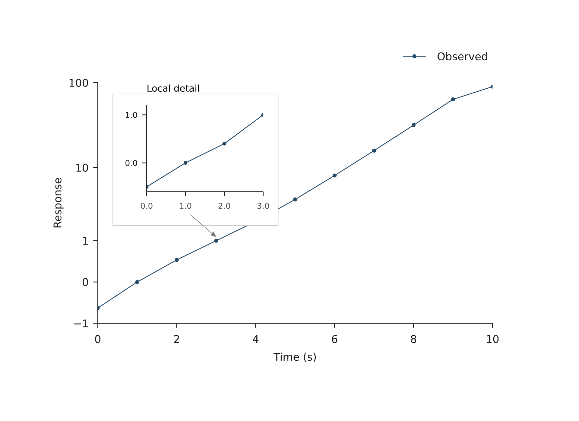
Source: inset.lay.
Reproduce: laymesh validate examples/plot/inset.lay; laymesh render examples/plot/inset.lay -o inset.png --dpi 150.
Observed CLI output: 有效:examples/plot/inset.lay(154 × 112 mm,1 个顶层实例); PNG 909 × 661 px at 150 DPI; warnings: none.
Polar and radar plots#
Directional curves and signed radii#
Compare mathematical angles with north/clockwise orientation; negative radii produce an expected suppressible warning.
page=canvas(size=(205 mm,120 mm),background="#ffffff")s=plot_style(font_family="DejaVu Sans",font_size=7 pt,grid_color="#dddddd")p=plot(projection="polar",size=(98 mm,100 mm),plot_area=box(offset=(18 mm, 18 mm), size=(62 mm, 62 mm)),style=s, theta=axis(ticks=[0,90,180,270],grid="major"),r=axis(range=(0,5),ticks=[1,3,5],grid="major",tick_font_size=6 pt))a=p.line(theta=[0,45,90,135,180,225,270,315],r=[4.5,3,1.6,2.5,4,2.8,1.3,3.4],closed=true,marker="diamond",marker_size=1.7 mm,color="#264b69",label="Response")p.line(theta=[350,10],r=[4,4],color="#b65337",line_width=0.6 mm,label="350 to 10 degrees")p.scatter(theta=[180],r=[-4.5],marker="circle",marker_size=3 mm,marker_fill="none",marker_border_color="#b65337",marker_border_width=0.3 mm)c=page.add(p,offset=(3 mm,4 mm))page.add(text(content="(a) Directional response",font_family="DejaVu Sans",font_size=9 pt),target=c.plot_top_left,offset=(-4 mm,-15 mm))page.add(text(content="Peak",font_family="DejaVu Sans",font_size=7 pt),target=c.data(theta=0,r=4.5),offset=(-12 mm,-6 mm))q=plot(projection="polar",size=(98 mm,100 mm),plot_area=box(offset=(18 mm, 18 mm), size=(62 mm, 62 mm)),style=s,theta_zero=90 deg,theta_direction="cw", theta=axis(ticks=[0,90,180,270],tick_text=["N","E","S","W"],grid="major"),r=axis(range=(0,5),ticks=[1,3,5],grid="major",tick_font_size=6 pt))q.line(theta=[0,45,90,135,180,225,270,315],r=[4.5,3,1.6,2.5,4,2.8,1.3,3.4],closed=true,marker="diamond",marker_size=1.7 mm,color="#264b69")d=page.add(q,offset=(103 mm,4 mm))page.add(text(content="(b) North / clockwise",font_family="DejaVu Sans",font_size=9 pt),target=d.plot_top_left,offset=(-4 mm,-15 mm))page.add(legend(layers=[a],style=s),offset=(12 mm,103 mm))page.add(text(content="Negative radius: same point after a half-turn (warning can be hidden).",font_family="DejaVu Sans",font_size=7 pt),offset=(53 mm,107 mm))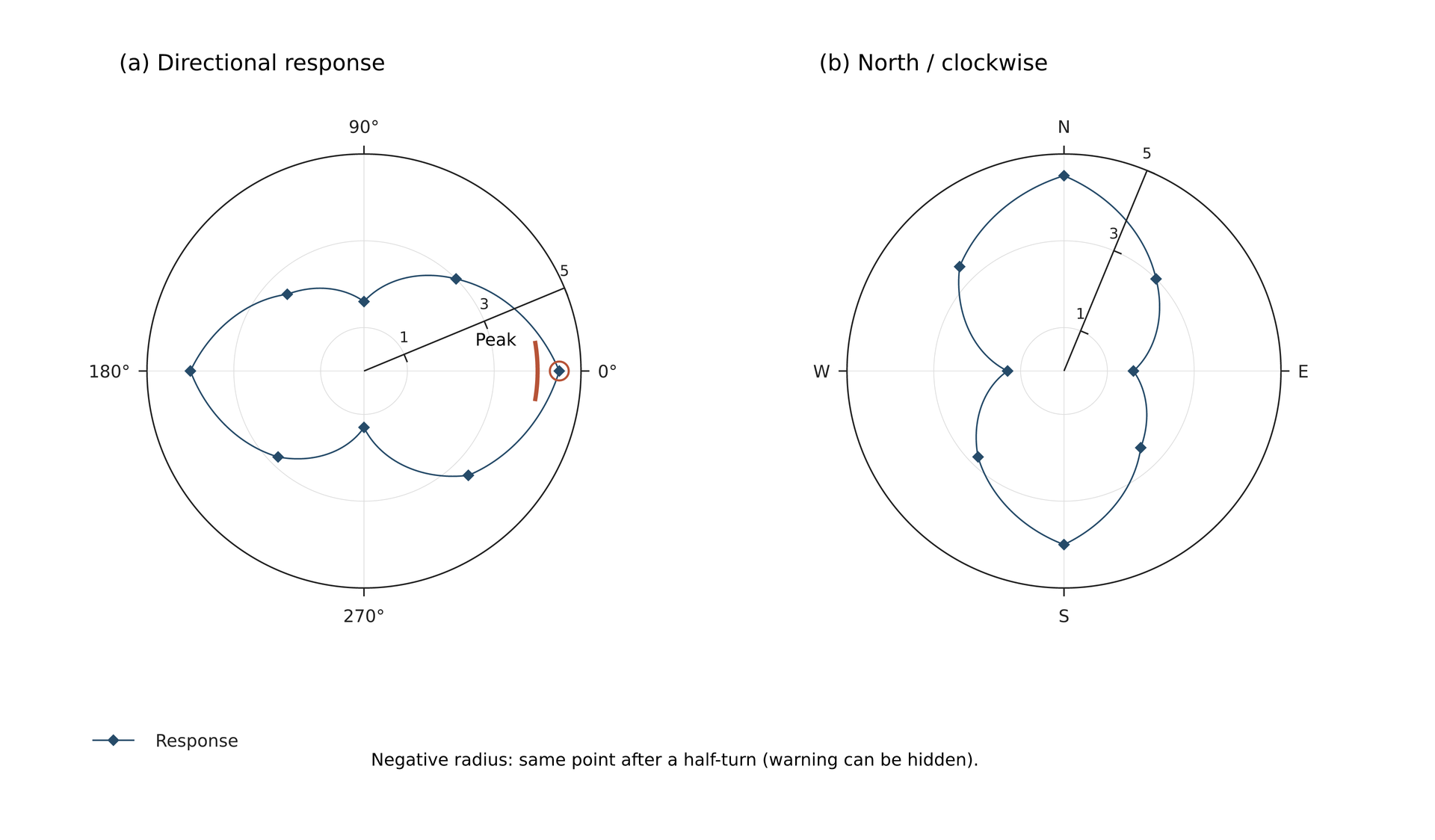
Source: polar-directions.lay.
Reproduce: laymesh validate examples/plot/polar-directions.lay; laymesh render examples/plot/polar-directions.lay -o polar-directions.png --dpi 150.
Observed CLI output: 有效:examples/plot/polar-directions.lay(205 × 120 mm,7 个顶层实例); PNG 1211 × 709 px at 150 DPI; warnings: examples/plot/polar-directions.lay:8:1: W_POLAR_NEGATIVE_RADIUS: 极坐标包含 1 个负半径坐标;已翻转半周并取绝对值.
Polar uncertainty and caps#
Radial/angular errors, hollow markers and physical hatching in a fixed sector.
page=canvas(size=(128 mm,112 mm),background="#ffffff")s=plot_style(font_family="DejaVu Sans",font_size=8 pt)p=plot(projection="polar",size=(118 mm,100 mm),plot_area=box(offset=(23 mm, 20 mm), size=(72 mm, 72 mm)),style=s, theta=axis(range=(0,240),ticks=[0,60,120,180,240],grid="major"),r=axis(range=(0,8),ticks=[2,4,6,8],grid="major",tick_font_size=6 pt))b=p.band(theta=[10,45,90,135,180,225],lower=[3,4,3,2,3,2],upper=[5,6,5,4,5,4],fill="#b3c5ce",hatch="slash",hatch_spacing=2 mm,hatch_width=0.1 mm,opacity=0.45,label="Uncertainty")e=p.errorbar(theta=[10,45,90,135,180,225],r=[4,5,4,3,4,3],thetaerr=6,rerr=0.5,marker="diamond",marker_size=2 mm,marker_fill="none",marker_border_color="#264b69",color="#264b69",cap_size=2 mm,label="Measurements")c=page.add(p,offset=(4 mm,2 mm))page.add(text(spans=[span("Signal "),formula(source=r"I(\theta)",font_size=10 pt)],font_family="DejaVu Sans",font_size=10 pt),offset=(30 mm,5 mm))page.add(legend(layers=[b,e],columns=2,style=s),offset=(20 mm,99 mm))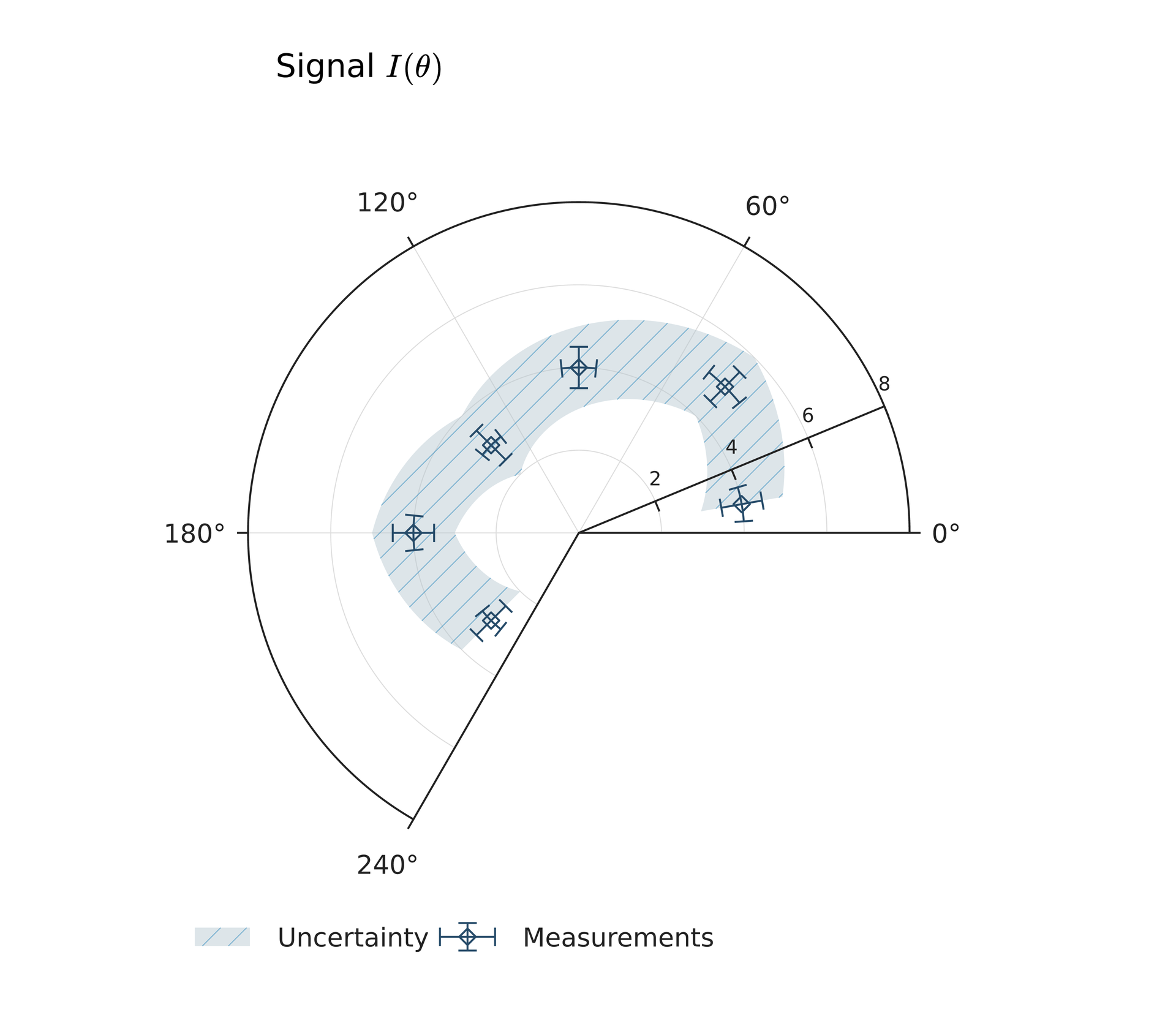
Source: polar-errors.lay.
Reproduce: laymesh validate examples/plot/polar-errors.lay; laymesh render examples/plot/polar-errors.lay -o polar-errors.png --dpi 150.
Observed CLI output: 有效:examples/plot/polar-errors.lay(128 × 112 mm,3 个顶层实例); PNG 756 × 661 px at 150 DPI; warnings: none.
Angular histograms and annular bars#
Periodic bins preserve counts; explicit baselines stack sectors around a physical inner hole.
page=canvas(size=(208 mm,116 mm),background="#ffffff")s=plot_style(font_family="DejaVu Sans",font_size=7 pt)p=plot(projection="polar",size=(100 mm,100 mm),plot_area=box(offset=(18 mm, 20 mm), size=(64 mm, 64 mm)),style=s,theta_zero=90 deg,theta_direction="cw", theta=axis(ticks=[0,90,180,270],grid="major"),r=axis(range=(0,8),ticks=[2,4,6,8],grid="major",tick_font_size=6 pt))p.hist(values=[-5,0,10,15,20,40,50,80,90,100,130,160,180,190,195,200,205,230,260,280,315,350,360],bins=8,fill="#8da9b9",border_color="#ffffff",border_width=0.25 mm)a=page.add(p,offset=(2 mm,2 mm))page.add(text(content="(a) Angular counts",font_family="DejaVu Sans",font_size=9 pt),target=a.plot_top_left,offset=(-3 mm,-15 mm))q=plot(projection="polar",size=(100 mm,100 mm),plot_area=box(offset=(18 mm, 20 mm), size=(64 mm, 64 mm)),style=s,inner_radius=7 mm, theta=axis(ticks=[0,90,180,270],grid="major"),r=axis(range=(0,8),ticks=[2,4,6,8],grid="major",tick_font_size=6 pt))u=q.bar(positions=[0,60,120,180,240,300],values=[3,4,2,5,3,4],angle_width=40,fill="#264b69",border_color="none",label="Series A")v=q.bar(positions=[0,60,120,180,240,300],values=[2,1,3,1,2,2],baseline=[3,4,2,5,3,4],angle_width=40,fill="#b46c50",border_color="none",label="Series B")b=page.add(q,offset=(105 mm,2 mm))page.add(text(content="(b) Explicit stacking / inner hole",font_family="DejaVu Sans",font_size=9 pt),target=b.plot_top_left,offset=(-8 mm,-15 mm))page.add(legend(layers=[u,v],columns=2,style=s),offset=(66 mm,102 mm))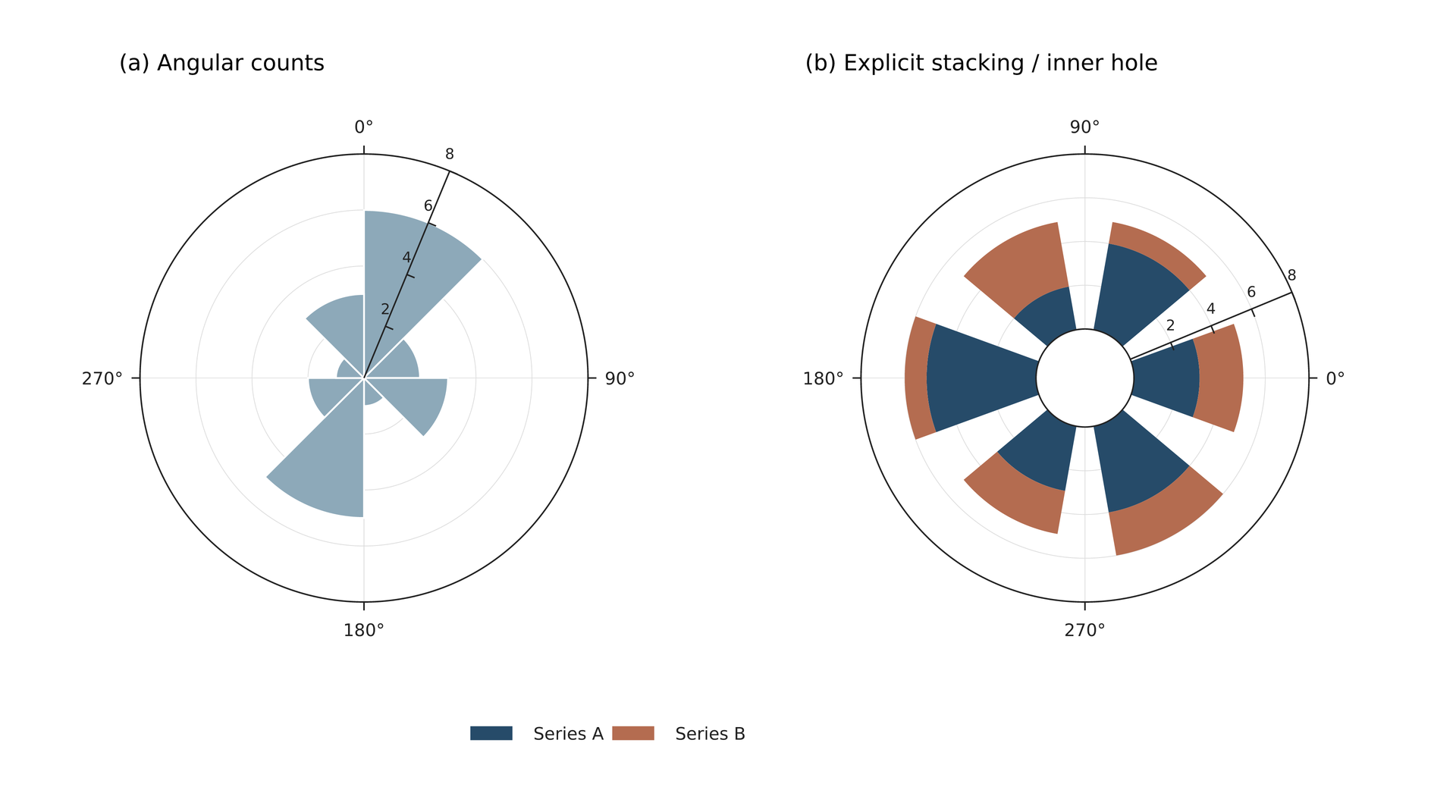
Source: polar-rose.lay.
Reproduce: laymesh validate examples/plot/polar-rose.lay; laymesh render examples/plot/polar-rose.lay -o polar-rose.png --dpi 150.
Observed CLI output: 有效:examples/plot/polar-rose.lay(208 × 116 mm,5 个顶层实例); PNG 1228 × 685 px at 150 DPI; warnings: none.
Polar cells and periodic contours#
Nonuniform radial cells and periodic contour fields share an independent colorbar.
page=canvas(size=(218 mm,127 mm),background="#ffffff")s=plot_style(font_family="DejaVu Sans",font_size=7 pt)colors=color_scale(vmin=0,vmax=4,cmap="viridis")p=plot(projection="polar",size=(102 mm,102 mm),plot_area=box(offset=(18 mm, 20 mm), size=(66 mm, 66 mm)),style=s, theta=axis(ticks=[0,90,180,270]),r=axis(range=(0,3),ticks=[1,2,3],tick_color="#ffffff",tick_font_size=6 pt))p.heatmap(z=[[1,1.1,1.2,1.1,1,0.9,0.8,0.9],[2,2.3,2.6,2.3,2,1.7,1.4,1.7],[3,3.4,3.8,3.4,3,2.6,2.2,2.6]],theta_edges=[0,45,90,135,180,225,270,315,360],r_edges=[0,0.8,1.8,3],color_scale=colors)a=page.add(p,offset=(4 mm,3 mm))page.add(text(content="(a) Nonuniform polar cells",font_family="DejaVu Sans",font_size=9 pt),target=a.plot_top_left,offset=(-6 mm,-16 mm))q=plot(projection="polar",size=(102 mm,102 mm),plot_area=box(offset=(18 mm, 20 mm), size=(66 mm, 66 mm)),style=s, theta=axis(ticks=[0,90,180,270]),r=axis(range=(0,3),ticks=[1,2,3],tick_color="#ffffff",tick_font_size=6 pt))z=[[0,0,0,0,0,0,0,0],[1,1.15,1.3,1.15,1,0.85,0.7,0.85],[2,2.3,2.6,2.3,2,1.7,1.4,1.7],[3,3.4,3.8,3.4,3,2.6,2.2,2.6]]q.contourf(z=z,theta=[0,45,90,135,180,225,270,315],r=[0,1,2,3],levels=[0,0.5,1,1.5,2,2.5,3,3.5],periodic=true,color_scale=colors)q.contour(z=z,theta=[0,45,90,135,180,225,270,315],r=[0,1,2,3],levels=[1,2,3],periodic=true,color="#ffffff",line_width=0.15 mm)b=page.add(q,offset=(112 mm,3 mm))page.add(text(content="(b) Periodic contour bands",font_family="DejaVu Sans",font_size=9 pt),target=b.plot_top_left,offset=(-6 mm,-16 mm))page.add(colorbar(scale=colors,orientation="horizontal",length=86 mm,thickness=3 mm,ticks=[0,1,2,3,4],label=formula(source=r"I(r,\theta)",font_size=9 pt),style=s),offset=(68 mm,104 mm))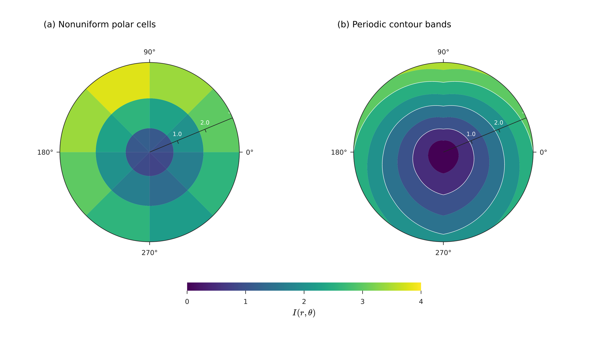
Source: polar-field.lay.
Reproduce: laymesh validate examples/plot/polar-field.lay; laymesh render examples/plot/polar-field.lay -o polar-field.png --dpi 150.
Observed CLI output: 有效:examples/plot/polar-field.lay(218 × 127 mm,5 个顶层实例); PNG 1287 × 750 px at 150 DPI; warnings: none.
Radar charts in original units#
Explicit indicator ranges retain signed raw units and anchors, alongside a common-scale example.
page=canvas(size=(238 mm,126 mm),background="#ffffff")s=plot_style(font_family="DejaVu Sans",font_size=7 pt)p=plot(projection="radar",size=(115 mm,110 mm),plot_area=box(offset=(25 mm, 25 mm), size=(64 mm, 64 mm)),style=s, categories=["Strength","Density","Cost","Temperature","Life"], category_labels=["Strength (MPa)","Density", "Cost", "Temperature (C)","Life"], ranges=[(0,1000),(0,10),(0,100),(-50,150),(0,100)],r=axis(ticks=[0.5,1],grid="major",tick_font_size=5 pt))a=p.area(values=[800,6,40,70,80],fill="#264b69",color="#264b69",opacity=0.18,label="Material A")b=p.area(values=[600,4,70,120,65],fill="#b46c50",color="#b46c50",opacity=0.18,label="Material B")p.line(values=[800,6,40,70,80],marker="diamond",marker_size=1.5 mm,color="#264b69")p.line(values=[600,4,70,120,65],marker="triangle",marker_size=1.5 mm,color="#b46c50")c=page.add(p,offset=(2 mm,0 mm))page.add(text(content="(a) Explicit ranges, original units",font_family="DejaVu Sans",font_size=9 pt),offset=(12 mm,5 mm))q=plot(projection="radar",size=(115 mm,110 mm),plot_area=box(offset=(25 mm, 25 mm), size=(64 mm, 64 mm)),style=s,categories=["A","B","C","D","E"],radar_frame="circle",r=axis(range=(0,1),ticks=[0.5,1],grid="major",tick_font_size=5 pt))q.area(values=[0.8,0.6,0.4,0.6,0.8],fill="#264b69",opacity=0.18)q.line(values=[0.8,0.6,0.4,0.6,0.8],marker="diamond",marker_size=1.5 mm,color="#264b69")d=page.add(q,offset=(120 mm,0 mm))page.add(text(content="(b) Common scale / circular frame",font_family="DejaVu Sans",font_size=9 pt),offset=(128 mm,5 mm))page.add(legend(layers=[a,b],columns=2,style=s),offset=(78 mm,108 mm))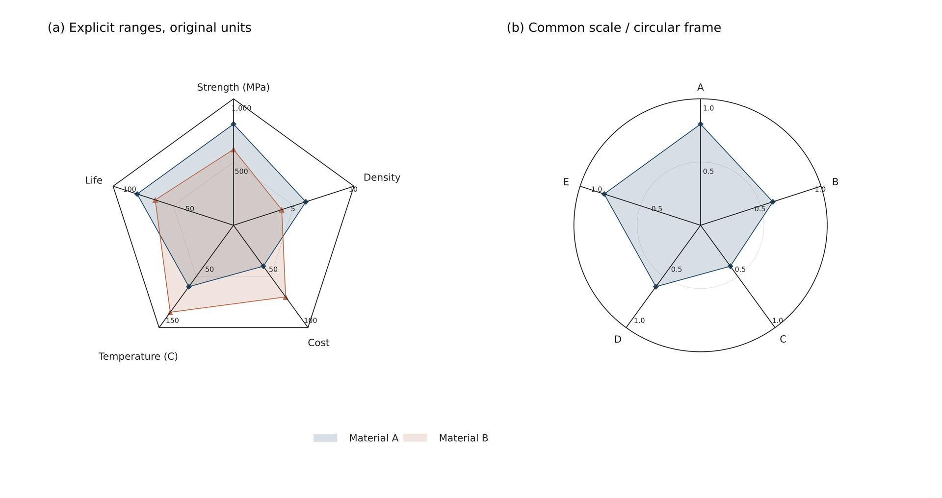
Source: radar.lay.
Reproduce: laymesh validate examples/plot/radar.lay; laymesh render examples/plot/radar.lay -o radar.png --dpi 150.
Observed CLI output: 有效:examples/plot/radar.lay(238 × 126 mm,5 个顶层实例); PNG 1406 × 744 px at 150 DPI; warnings: none.
Polar and radar data from Python#
NumPy fields/radar arrays persist as hashed JSON; missing adjacent grid cells remain empty.
page=canvas(size=(228 mm,132 mm),background="#ffffff")s=plot_style(font_family="DejaVu Sans",font_size=7 pt)colors=color_scale(vmin=0,vmax=4,cmap="viridis")p=plot(projection="polar",size=(105 mm,110 mm),plot_area=box(offset=(20 mm, 22 mm), size=(66 mm, 66 mm)),style=s, theta=axis(ticks=[0,90,180,270]),r=axis(range=(0,3),ticks=[1,2,3],tick_color="#ffffff",tick_font_size=6 pt))p.contourf(z=array(src="polar-data.assets/field-1f0c1f4eca6acc4d.json"),theta=array(src="polar-data.assets/theta-a1a6d05666acec02.json"),r=array(src="polar-data.assets/radius-c2faeb8428cb0845.json"),levels=[0,0.5,1,1.5,2,2.5,3,3.5],periodic=true,color_scale=colors)a=page.add(p,offset=(3 mm,0 mm))page.add(text(content="(a) Missing polar samples",font_family="DejaVu Sans",font_size=9 pt),offset=(13 mm,5 mm))q=plot(projection="radar",size=(118 mm,110 mm),plot_area=box(offset=(25 mm, 22 mm), size=(66 mm, 66 mm)),style=s, categories=["Strength","Density","Cost","Temperature","Life"],ranges=[(0,1000),(0,10),(0,100),(-50,150),(0,100)],r=axis(ticks=[0.5,1],grid="major",tick_font_size=5 pt))q.area(values=array(src="polar-data.assets/values-24bfdcd1baba759e.json"),fill="#264b69",opacity=0.2)q.line(values=array(src="polar-data.assets/values-24bfdcd1baba759e.json"),color="#264b69",marker="diamond",marker_size=1.6 mm)b=page.add(q,offset=(109 mm,0 mm))page.add(text(content="(b) Raw units from Python",font_family="DejaVu Sans",font_size=9 pt),offset=(126 mm,5 mm))page.add(colorbar(scale=colors,orientation="horizontal",length=72 mm,thickness=3 mm,ticks=[0,1,2,3,4],label="Field",style=s),offset=(27 mm,107 mm))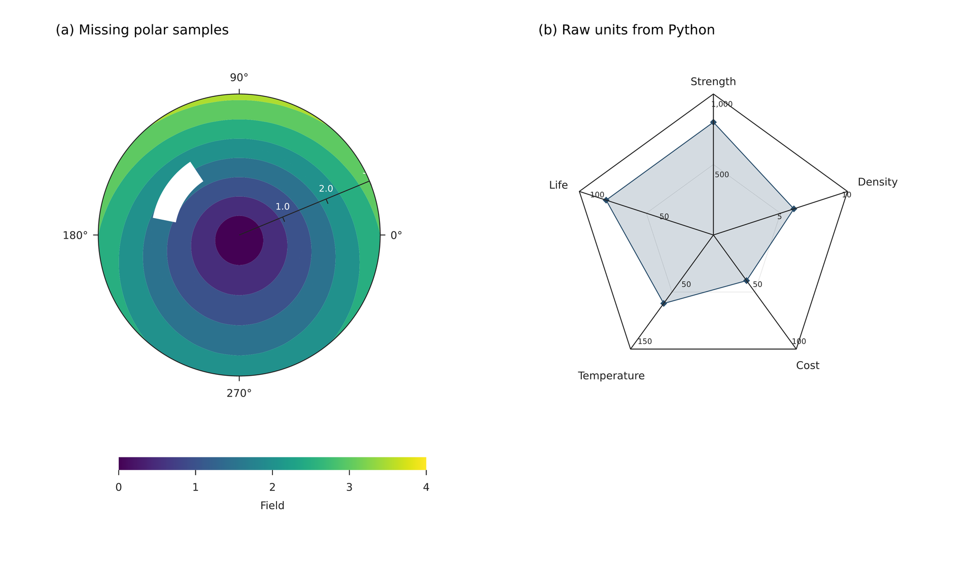
Source: polar-data.lay.
Reproduce: laymesh validate examples/plot/polar-data.lay; laymesh render examples/plot/polar-data.lay -o polar-data.png --dpi 150.
Observed CLI output: 有效:examples/plot/polar-data.lay(228 × 132 mm,5 个顶层实例); PNG 1346 × 780 px at 150 DPI; warnings: examples/plot/polar-data.lay:8:1: W_PLOT_MISSING: 等高线包含 9 个缺失采样点;邻接网格单元留空.
Plot series from a dictionary#
series.items() supplies legend names and data; palette("tab10") drives automatic color rotation.
# Loop through series in insertion order; style colors rotate automatically.page=canvas(size=(130mm,90mm),background="#ffffff")series={"Baseline":[1,2,3,3.5],"Annealed":[1.2,2.8,3.1,4],"Cold worked":[2,2.2,2.8,3.1]}style=plot_style(colors=palette("tab10"),font_family="DejaVu Sans",font_size=8pt)chart=plot(size=(120mm,80mm),style=style,x=axis(label="Time",range=(0,3)),y=axis(label="Response",range=(0,5)))for name,ys in series.items() { chart.line(x=[0,1,2,3],y=ys,label=name,marker="circle")}chart.legend(position="top_left")page.add(chart,offset=(5mm,5mm))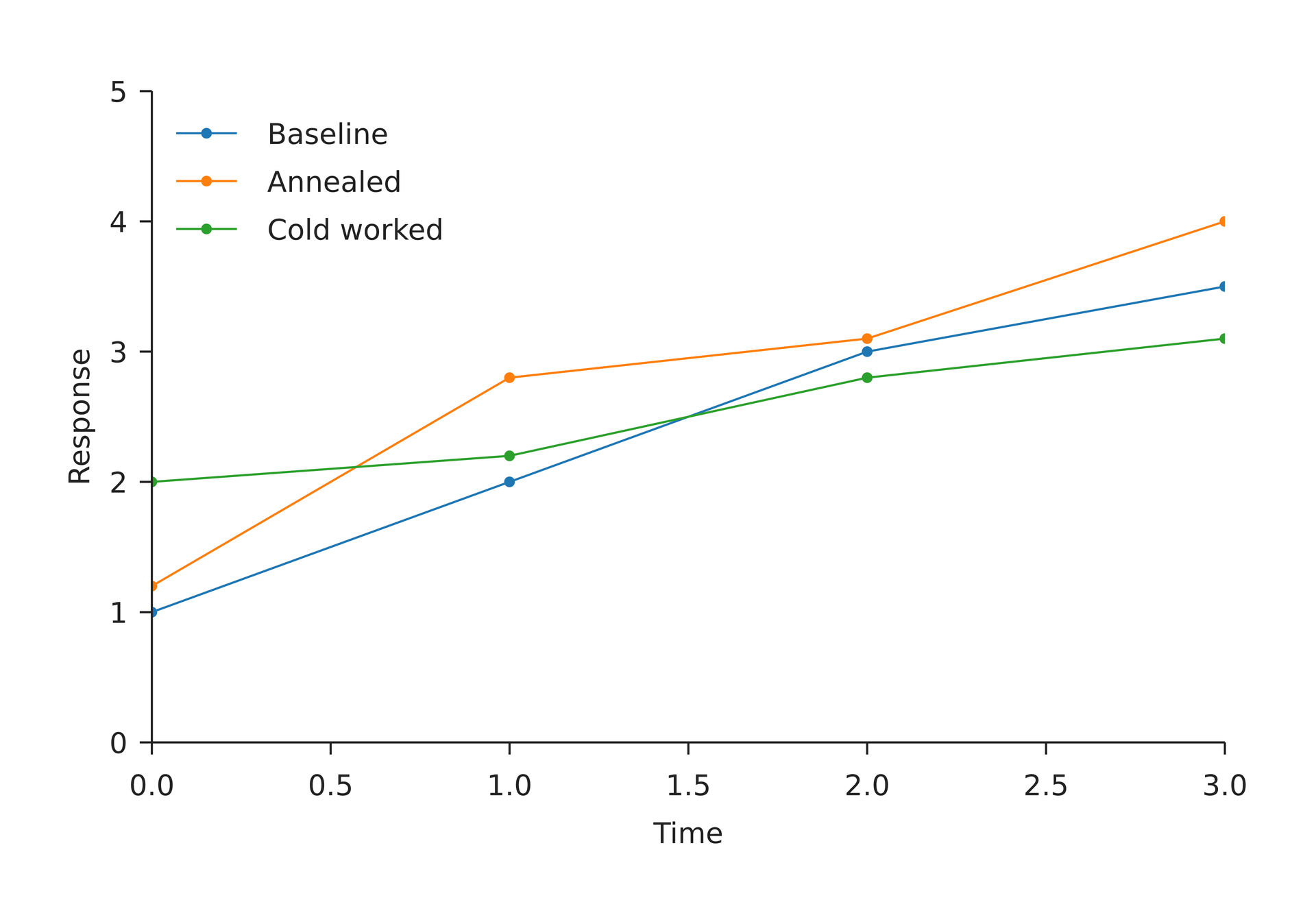
Source: dictionary-series.lay.
Reproduce: laymesh validate examples/plot/dictionary-series.lay; laymesh render examples/plot/dictionary-series.lay -o dictionary-series.png --dpi 150.
Observed CLI output: 有效:examples/plot/dictionary-series.lay(130 × 90 mm,1 个顶层实例); PNG 768 × 531 px, 150 DPI.
Complete colormap catalogue#
All 87 canonical Matplotlib 3.11.2 presets; qualitative maps retain their native color order.
# Complete canonical preset catalogue; aliases and _r variants are omitted here.names=cmap_names()page=canvas(size=(210mm,len(names)*4mm+22mm),background="#ffffff")page.add(text(content="Matplotlib 3.11.2 - 87 cmap presets",font_family="DejaVu Sans",font_size=12pt),offset=(8mm,5mm))for row,name in enumerate(names) { cm=cmap(name) colors=cm.colors(64) if cm.category=="qualitative" {colors=cm.colors()} width=142mm/len(colors) page.add(text(content=name,font_family="DejaVu Sans",font_size=7pt),offset=(8mm,18mm+row*4mm)) for i,color in enumerate(colors) { page.add(rect(size=(width,3mm),fill=color),offset=(57mm+i*width,18mm+row*4mm)) }}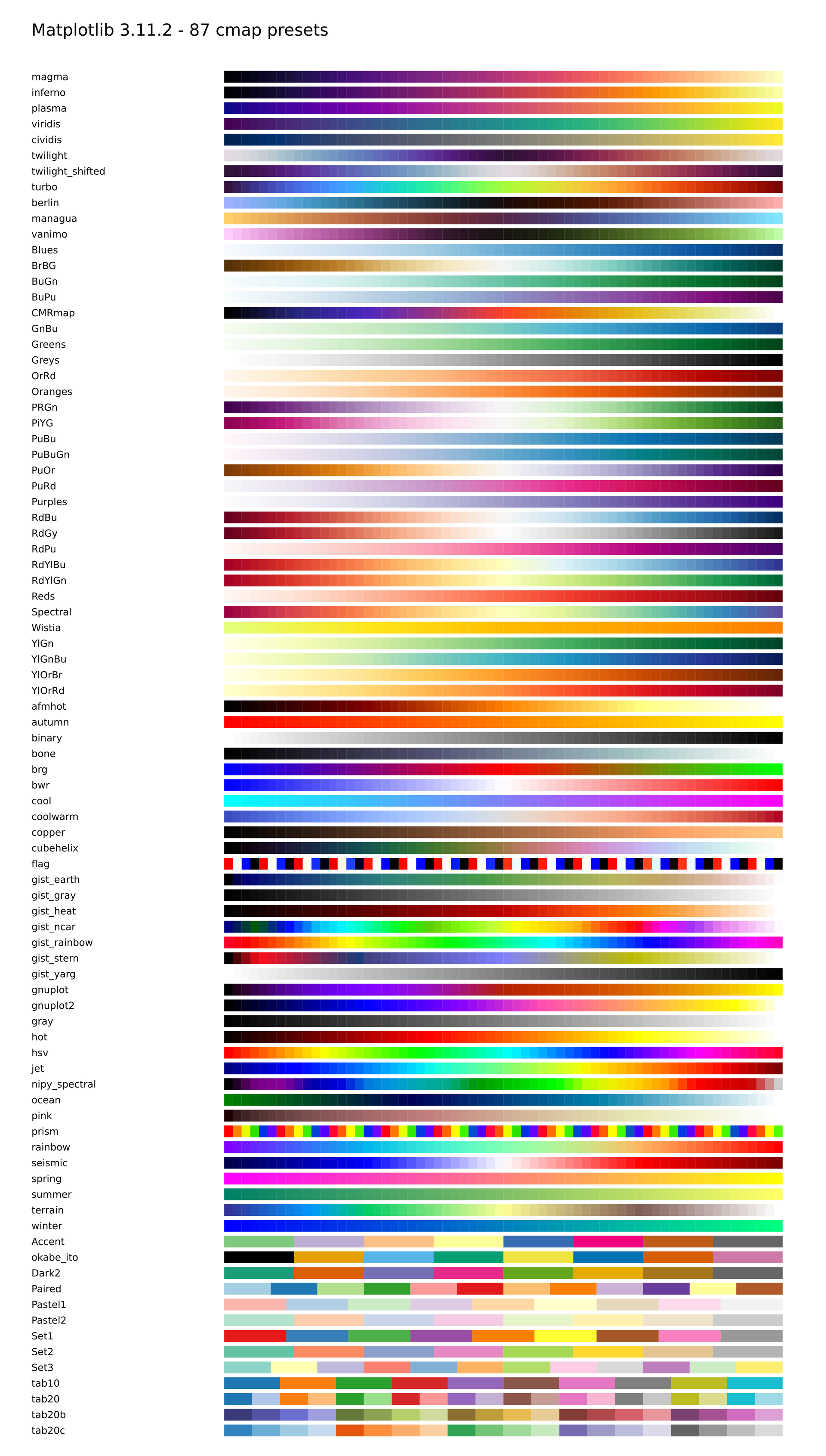
Source: cmap-presets.lay.
Reproduce: laymesh validate examples/plot/cmap-presets.lay; laymesh render examples/plot/cmap-presets.lay -o cmap-presets.png --dpi 150.
Observed CLI output: 有效:examples/plot/cmap-presets.lay(210 × 370 mm,4976 个顶层实例); PNG 1240 × 2185 px, 150 DPI.
Shared colormap and colorbar#
One immutable coolwarm handle supplies the heatmap, filled contours, scatter points and shared colorbar.
# The same immutable handle drives heatmap, contour, scatter and colorbar.page=canvas(size=(210mm,108mm),background="#ffffff")cm=cmap("coolwarm")scale=color_scale(norm="centered",vmin=-2,vmax=2,center=0,cmap=cm)style=plot_style(font_family="DejaVu Sans",font_size=8pt)a=plot(size=(90mm,85mm),style=style,x=axis(range=(0,4)),y=axis(range=(0,4)))a.heatmap(z=[[-2,-1,0,1],[-1,0,1,2],[0,1,2,1],[1,2,1,0]],extent=(0,4,0,4),color_scale=scale)page.add(a,offset=(4mm,5mm))b=plot(size=(90mm,85mm),style=style,x=axis(range=(0,4)),y=axis(range=(0,4)))b.contourf(z=[[-2,-1,0,1,2],[-1,0,1,2,1],[0,1,2,1,0],[1,2,1,0,-1],[2,1,0,-1,-2]],levels=[-2,-1,0,1],color_scale=scale)b.scatter(x=[0.5,1.5,2.5,3.5],y=[3.5,2.5,1.5,0.5],c=[-2,-1,1,2],color_scale=scale,marker_border_color="#222222",marker_border_width=0.5pt)page.add(b,offset=(101mm,5mm))page.add(colorbar(scale=scale,length=150mm,orientation="horizontal",label="Shared value",style=style),offset=(28mm,90mm))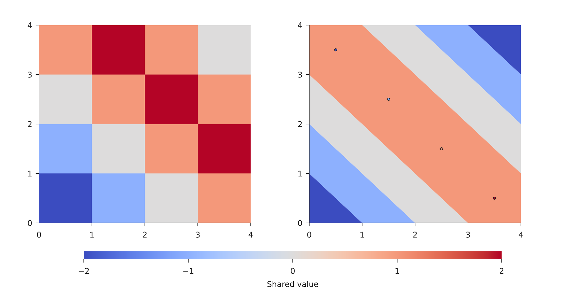
Source: cmap-scales.lay.
Reproduce: laymesh validate examples/plot/cmap-scales.lay; laymesh render examples/plot/cmap-scales.lay -o cmap-scales.png --dpi 150.
Observed CLI output: 有效:examples/plot/cmap-scales.lay(210 × 108 mm,3 个顶层实例); PNG 1240 × 638 px, 150 DPI.