误差棒与填充带#

用途与概念#

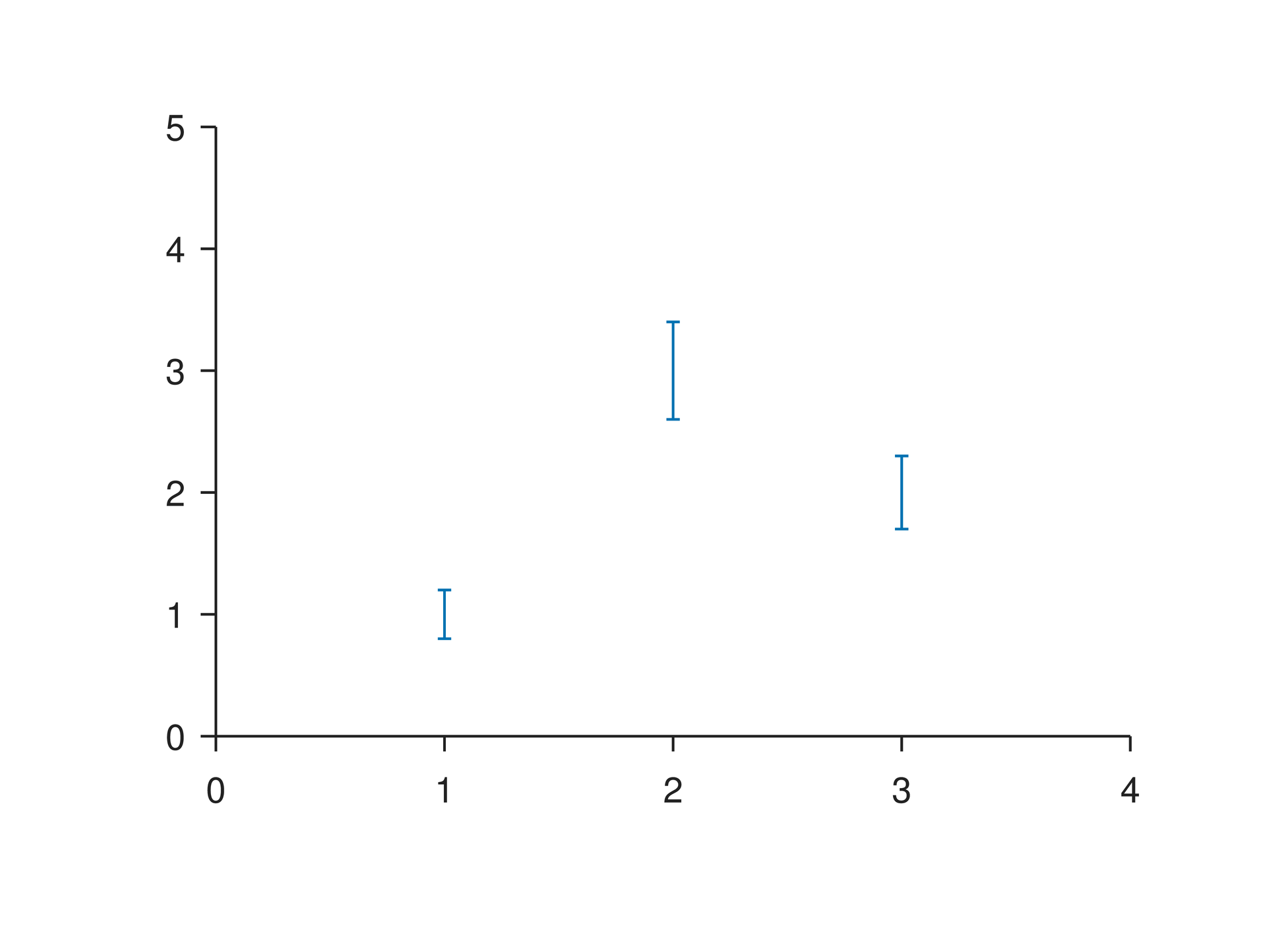
errorbar 在采样点绘制 xerr/yerr 不确定度，band 在 x 对应的 lower/upper 之间填充。误差是数据单位，cap_size 和线宽是物理长度。

最小完整示例#

此文件包含画布及必要定义，可直接运行 laymesh validate 或 laymesh render，不依赖前文未声明的变量。

1# Minimal complete example: plot.errorbar2page=canvas(size=(100mm,75mm),background="#ffffff")3p=plot(size=(86mm,62mm),x=axis(range=(0,4)),y=axis(range=(0,5)))4p.errorbar(x=[1,2,3],y=[1,3,2],yerr=[0.2,0.4,0.3])5page.add(p,offset=(7mm,6mm))

# Minimal complete example: plot.errorbar
page=canvas(size=(100mm,75mm),background="#ffffff")
p=plot(size=(86mm,62mm),x=axis(range=(0,4)),y=axis(range=(0,5)))
p.errorbar(x=[1,2,3],y=[1,3,2],yerr=[0.2,0.4,0.3])
page.add(p,offset=(7mm,6mm))

1# Minimal complete example: plot.errorbar2page=canvas(size=(100mm,75mm),background="#ffffff")3p=plot(size=(86mm,62mm),x=axis(range=(0,4)),y=axis(range=(0,5)))4p.errorbar(x=[1,2,3],y=[1,3,2],yerr=[0.2,0.4,0.3])5page.add(p,offset=(7mm,6mm))

# Minimal complete example: plot.errorbar
page=canvas(size=(100mm,75mm),background="#ffffff")
p=plot(size=(86mm,62mm),x=axis(range=(0,4)),y=axis(range=(0,5)))
p.errorbar(x=[1,2,3],y=[1,3,2],yerr=[0.2,0.4,0.3])
page.add(p,offset=(7mm,6mm))

依赖文件

examples/manual/plot-errorbar.lay

参数与默认行为#

裸几何长度使用画布单位，裸字号和描边宽度使用 pt。显式调用参数优先于继承和主题默认值；下面的接口参考逐项列出允许类型、可选值与默认来源。

组合用法#

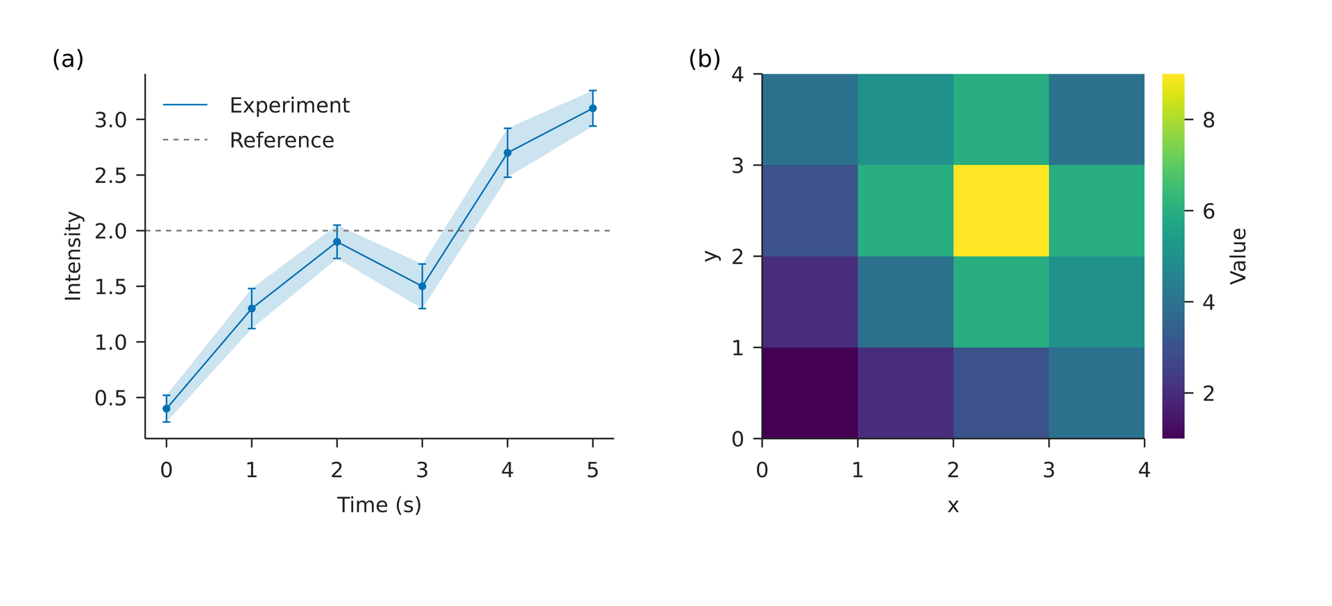
同一实验数据可组合半透明 band、中心折线及点误差。误差可对称或分别指定上下误差；上下界须与采样位置对应。

1page = canvas(size=(180 mm, 82 mm), background="#ffffff")2d = table(src="results.csv")3style = plot_style(font_family="DejaVu Sans", font_size=8 pt, line_width=0.6 pt)4p = plot(size=(80 mm, 65 mm), x=axis(label="Time (s)"), y=axis(label="Intensity"), style=style)5p.band(x=d["time"], lower=d["lower"], upper=d["upper"], color="#0072B2")6p.line(x=d["time"], y=d["signal"], color="#0072B2", label="Experiment")7p.scatter(x=d["time"], y=d["signal"], color="#0072B2", marker_size=3 pt)8p.errorbar(x=d["time"], y=d["signal"], yerr=d["error"], color="#0072B2")9p.hline(y=2, color="#777777", line_dash=[2 pt, 2 pt], label="Reference")10p.legend(position= top_left)11left = page.add(p, target=page.top_left, offset=(7 mm, 6 mm))12h = plot(size=(80 mm, 65 mm), x=axis(label="x"), y=axis(label="y"), style=style)13heat = h.heatmap(z=[[1,2,3,4],[2,4,6,5],[3,6,9,6],[4,5,6,4]], extent=(0,4,0,4), origin= lower, cmap="viridis")14h.colorbar(heat, label="Value")

page = canvas(size=(180 mm, 82 mm), background="#ffffff")
d = table(src="results.csv")
style = plot_style(font_family="DejaVu Sans", font_size=8 pt, line_width=0.6 pt)
p = plot(size=(80 mm, 65 mm), x=axis(label="Time (s)"), y=axis(label="Intensity"), style=style)
p.band(x=d["time"], lower=d["lower"], upper=d["upper"], color="#0072B2")
p.line(x=d["time"], y=d["signal"], color="#0072B2", label="Experiment")
p.scatter(x=d["time"], y=d["signal"], color="#0072B2", marker_size=3 pt)
p.errorbar(x=d["time"], y=d["signal"], yerr=d["error"], color="#0072B2")
p.hline(y=2, color="#777777", line_dash=[2 pt, 2 pt], label="Reference")
p.legend(position= top_left)
left = page.add(p, target=page.top_left, offset=(7 mm, 6 mm))
h = plot(size=(80 mm, 65 mm), x=axis(label="x"), y=axis(label="y"), style=style)
heat = h.heatmap(z=[[1,2,3,4],[2,4,6,5],[3,6,9,6],[4,5,6,4]], extent=(0,4,0,4), origin= lower, cmap="viridis")
h.colorbar(heat, label="Value")

1page = canvas(size=(180 mm, 82 mm), background="#ffffff")2d = table(src="results.csv")3style = plot_style(font_family="DejaVu Sans", font_size=8 pt, line_width=0.6 pt)4p = plot(size=(80 mm, 65 mm), x=axis(label="Time (s)"), y=axis(label="Intensity"), style=style)5p.band(x=d["time"], lower=d["lower"], upper=d["upper"], color="#0072B2")6p.line(x=d["time"], y=d["signal"], color="#0072B2", label="Experiment")7p.scatter(x=d["time"], y=d["signal"], color="#0072B2", marker_size=3 pt)8p.errorbar(x=d["time"], y=d["signal"], yerr=d["error"], color="#0072B2")9p.hline(y=2, color="#777777", line_dash=[2 pt, 2 pt], label="Reference")10p.legend(position= top_left)11left = page.add(p, target=page.top_left, offset=(7 mm, 6 mm))12h = plot(size=(80 mm, 65 mm), x=axis(label="x"), y=axis(label="y"), style=style)13heat = h.heatmap(z=[[1,2,3,4],[2,4,6,5],[3,6,9,6],[4,5,6,4]], extent=(0,4,0,4), origin= lower, cmap="viridis")14h.colorbar(heat, label="Value")15right = page.add(h, target=left.top_right, offset=(6 mm, 0 mm))16page.add(text(content="(a)", font_family="DejaVu Sans", font_size=9 pt), target=left.top_left)17page.add(text(content="(b)", font_family="DejaVu Sans", font_size=9 pt), target=right.top_left)

page = canvas(size=(180 mm, 82 mm), background="#ffffff")
d = table(src="results.csv")
style = plot_style(font_family="DejaVu Sans", font_size=8 pt, line_width=0.6 pt)
p = plot(size=(80 mm, 65 mm), x=axis(label="Time (s)"), y=axis(label="Intensity"), style=style)
p.band(x=d["time"], lower=d["lower"], upper=d["upper"], color="#0072B2")
p.line(x=d["time"], y=d["signal"], color="#0072B2", label="Experiment")
p.scatter(x=d["time"], y=d["signal"], color="#0072B2", marker_size=3 pt)
p.errorbar(x=d["time"], y=d["signal"], yerr=d["error"], color="#0072B2")
p.hline(y=2, color="#777777", line_dash=[2 pt, 2 pt], label="Reference")
p.legend(position= top_left)
left = page.add(p, target=page.top_left, offset=(7 mm, 6 mm))
h = plot(size=(80 mm, 65 mm), x=axis(label="x"), y=axis(label="y"), style=style)
heat = h.heatmap(z=[[1,2,3,4],[2,4,6,5],[3,6,9,6],[4,5,6,4]], extent=(0,4,0,4), origin= lower, cmap="viridis")
h.colorbar(heat, label="Value")
right = page.add(h, target=left.top_right, offset=(6 mm, 0 mm))
page.add(text(content="(a)", font_family="DejaVu Sans", font_size=9 pt), target=left.top_left)
page.add(text(content="(b)", font_family="DejaVu Sans", font_size=9 pt), target=right.top_left)

1time,signal,error,lower,upper20,0.4,0.12,0.28,0.5231,1.3,0.18,1.12,1.4842,1.9,0.15,1.75,2.0553,1.5,0.20,1.30,1.7064,2.7,0.22,2.48,2.9275,3.1,0.16,2.94,3.26

time,signal,error,lower,upper
0,0.4,0.12,0.28,0.52
1,1.3,0.18,1.12,1.48
2,1.9,0.15,1.75,2.05
3,1.5,0.20,1.30,1.70
4,2.7,0.22,2.48,2.92
5,3.1,0.16,2.94,3.26